

Fiber_Optics_Physics_Technology
.pdf9.3. Nonlinear Wave Equation |
157 |
In order to insert Eq. (9.10) in Eq. (9.9), we first take the derivatives:
|
|
|
|
∂E |
= |
|
∂A |
ei(ω0t−β0z) |
|
|
|
|
|
|
|
|
|
|
|
|
||||||||||||
|
|
|
|
|
∂x |
|
|
|
|
|
|
|
|
|
|
|
|
|
|
|
||||||||||||
|
|
|
|
|
|
|
∂x |
|
|
|
|
|
|
|
|
|
|
|
|
|
|
|
|
|
|
|||||||
|
|
|
|
∂2E |
= |
∂2A |
ei(ω0t−β0z) |
|
|
|
|
|
|
|
|
|
|
|
|
|||||||||||||
|
|
|
|
|
∂x2 |
|
|
∂x2 |
|
|
|
|
|
|
|
|
|
|
|
|
||||||||||||
|
|
|
|
|
|
|
|
|
|
|
|
|
|
|
|
|
|
|
|
|
|
|
|
|||||||||
|
|
|
|
∂E |
= |
|
∂A |
ei(ω0t−β0z) |
|
|
|
|
|
|
|
|
|
|
|
|
||||||||||||
|
|
|
|
|
∂y |
|
|
|
|
|
|
|
|
|
|
|
|
|
|
|
||||||||||||
|
|
|
|
|
|
|
∂y |
|
|
|
|
|
|
|
|
|
|
|
|
|
|
|
|
|
|
|||||||
|
|
|
|
∂2E |
= |
∂2A |
ei(ω0t−β0z) |
|
|
|
|
|
|
|
|
|
|
|
|
|||||||||||||
|
|
|
|
|
∂y2 |
|
|
∂y2 |
|
|
|
|
|
|
|
|
|
|
|
|
|
|||||||||||
|
|
|
|
|
|
|
|
|
|
|
|
|
|
|
|
|
|
|
|
|
|
|
|
|
||||||||
|
|
|
|
∂E |
= |
∂A |
ei(ω0t−β0z) − iβ0A ei(ω0t−β0z) |
|
|
|
||||||||||||||||||||||
|
|
|
|
|
|
|
|
|
|
|
|
|
|
|
||||||||||||||||||
|
|
|
|
|
∂z |
|
∂z |
|
|
|
||||||||||||||||||||||
|
|
|
|
∂2E |
= |
|
∂2A |
− |
2iβ0 |
∂A |
− |
β2A ei(ω0t−β0z) |
|
|
|
|||||||||||||||||
|
|
|
|
|
∂z2 |
|
∂z2 |
∂z |
|
|
|
|||||||||||||||||||||
|
|
|
|
|
|
|
|
|
|
0 |
|
|
|
|
|
|
|
|
||||||||||||||
|
|
|
|
∂E |
= |
|
∂A |
ei(ω0t−β0z) + iω0A ei(ω0t−β0z) |
|
|
|
|||||||||||||||||||||
|
|
|
|
|
∂t |
|
|
|
|
|
||||||||||||||||||||||
|
|
|
|
|
|
|
∂t |
|
|
|
|
|
|
|
|
|
|
|
|
|
|
|
|
|
|
|||||||
|
|
|
|
∂2E |
= |
|
∂2A |
+ 2iω0 |
∂A |
− |
ω2A ei(ω0t−β0z). |
|
|
|
||||||||||||||||||
|
|
|
|
|
∂t2 |
|
∂t2 |
∂t |
|
|
|
|||||||||||||||||||||
|
|
|
|
|
|
|
|
|
|
|
0 |
|
|
|
|
|
|
|
|
|||||||||||||
Now we insert |
|
|
|
|
|
|
|
|
|
|
|
|
|
|
|
|
|
|
|
|
|
|
|
|
||||||||
∂A |
|
∂2A |
∂2A |
∂2A |
|
|
|
n2 ∂2A |
n2 ∂A |
n2 |
||||||||||||||||||||||
−2iβ0 |
|
+ |
|
|
+ |
|
+ |
|
|
− β02A − |
|
|
|
− 2iω0 |
|
|
|
|
+ ω02 |
|
A = 0. |
|||||||||||
∂z |
∂x2 |
∂y2 |
|
∂z2 |
c2 |
∂t2 |
c2 |
∂t |
c2 |
|||||||||||||||||||||||
Obviously the exponential factor is cancelled out, and we succeeded in finding an equation of motion for the envelope! The two terms proportional to A mutually cancel because β02 = ω02n2/c2. The derivatives in x and y directions can be combined using the transverse nabla operator xy . Then this is what remains:
−2iβ0 |
∂A |
+ xy2 |
A + |
∂2A |
− |
n2 ∂2A |
− 2iω0 |
n2 ∂A |
= 0. |
(9.11) |
||||
∂z |
∂z2 |
c2 |
|
∂t2 |
c2 |
|
∂t |
|||||||
The kth derivative is of order k 1; therefore, in leading order we only retain
2iβ0 |
∂A |
|
+ 2iω0 |
n2 ∂A |
= 0 |
|||||||
|
|
|
|
|
|
|||||||
∂z |
|
c2 ∂t |
||||||||||
|
|
|
|
|
|
|||||||
or |
∂A |
|
n |
|
∂A |
|
|
|
|
|||
|
+ |
|
= 0. |
(9.12) |
||||||||
|
∂z |
|
|
|||||||||
|
|
c ∂t |
|
|||||||||
This describes an envelope which propagates with constant shape and with velocity v = c/n, the phase velocity. This is no wonder – we have neglected both dispersion and nonlinearity so far!
Indeed the equation is better than valid only in first order. In Eq. (9.12), we note that a z derivative of A (not of E!) is the same as a t derivative up to a factor of −n/c. One can do the same trick twice:
∂2A |
= |
|
n |
2 |
∂2A |
. |
2 |
|
2 |
||||
∂z |
− c ∂t |
|||||
158 Chapter 9. Basics of Nonlinearity
Now one sees that the third and fourth term in Eq. (9.11) cancel out. At next higher order this is what remains:
∂A |
+ |
n ∂A |
+ |
i |
xy2 A = 0. |
(9.13) |
|||
|
|
|
|
|
|
||||
∂z |
|
c ∂t |
2β0 |
||||||
This is di erent only in the term for transverse change. In a fiber, di raction is compensated by the waveguiding mechanism so that derivatives with respect to x and y are zero.
The term containing the first temporal derivative can be scaled out. To do
so we introduce a comoving frame of reference |
|
||||||
|
|
|
|
n |
|
||
|
|
τ = t − |
|
z |
|
||
|
|
c |
|
||||
and obtain |
|
|
|
|
|
|
|
∂A |
+ |
i |
|
||||
|
|
|
xy2 A = 0. |
(9.14) |
|||
|
∂z |
2β0 |
|||||
This equation describes the transverse di raction of a wave packet. Without transverse change the pulse shape is constant.
In a linear fiber, free from dispersion and loss, a wave packet propagates without change of shape with a velocity equal to the phase velocity.
Now we must incorporate the e ects of dispersion, loss, and nonlinearity. This implies that n will now become a function of frequency (or wavelength) and power (or amplitude), and the amplitude a function of position (or distance).
9.3.2Introducing Dispersion by a Fourier Technique
A Fourier transform is used to convert from a function in the temporal domain to the corresponding function in the frequency domain (or vice versa), or from spatial position to spatial frequency, etc. Let us begin with a time-frequency transformation of some function F (t, z).
We use the abbreviation
˜
F (ω) = FT F (t)
to denote the Fourier transform FT . . . , spelled out as
+∞
˜ iωt
F (ω) = F (t) e dt.
−∞
Then it holds that |
|
|
|
|
|
|
|
|
||
|
|
FT i |
∂ |
F (t) = +∞i |
∂F (t) |
eiωt dt. |
|
|
||
|
|
|
|
|||||||
|
|
|
∂t |
|
−∞ |
∂t |
|
|
||
By partial integration one finds: |
|
|
|
|
||||||
|
+∞iF (t) ∂ eiωtdt |
|||||||||
FT i ∂ F (t) |
= |
ieiωt F (t) +∞ |
||||||||
|
|
|
|
|
|
|
− |
|
|
|
∂t |
|
|
|
|
∂t |
|||||
|
|
|
|
|
|
+ −∞ |
−∞ |
|
|
|
|
|
|
= |
0 + ω |
∞F (t) eiωt dt |
|
|
|||
|
|
|
|
|
|
−∞ |
|
|
|
|
|
|
|
= |
ω FT F (t) |
|
|
|
|
||
|
|
|
= |
˜ |
|
|
|
|
|
|
|
|
|
ω F (ω). |
|
|
|
|
|||
9.3. Nonlinear Wave Equation |
159 |
In the second line, we assumed that F (t = ±∞) = 0, which means that for distant times F (t) decays. Then we conclude that a Fourier transform acts simply to replace
˜ |
↔ F (t), |
|
|||||
F (ω) |
|
||||||
˜ |
|
|
∂ |
|
|||
ωF (ω) |
↔ |
i |
∂t |
F (t), |
|||
ωk F˜(ω) |
↔ |
i |
∂ |
k |
F (t). |
||
|
|||||||
|
|
|
∂t |
|
|||
A factor ω in the frequency domain corresponds to an operator i(∂/∂t) in the time domain. The same logic applies also if instead of ω we use ω = ω − ω0 throughout, with fixed ω0.
Quite similarly we can do a position–spatial frequency transformation, i.e., a transformation between coordinate z and wave number β.
F˜(β) = FT F (z) |
= +∞F (z) e−iβz dt. |
|
|
|
−∞ |
The sign in the exponent stands for a wave traveling “to the right” or toward positive z. With an analogous calculation one finds the following correspondence:
˜ |
↔ F (z), |
|
||||||
F (β) |
|
|||||||
˜ |
|
|
∂ |
|
||||
βF (β) |
↔ −i |
∂z |
F (z), |
|||||
βk F˜(β) |
|
− |
i |
∂ |
k |
F (z). |
||
|
||||||||
|
↔ |
|
∂z |
|
||||
Again, this is also valid if β = β − β0 instead of β. We will now apply this insight to the series expansion of the wave number as a function of frequency, which is
β = β0 + ωβ1 + ω2 |
β2 |
+ |
ω3 |
β3 |
+ ··· . |
(9.15) |
2 |
6 |
Now we make the transition to the time domain by inserting operators and apply them to A(z, t):
|
|
β |
= |
β1 ω + |
|
β2 |
|
ω2 + |
β3 |
ω3 + ··· |
(9.16) |
|||||||||
|
|
|
2 |
|
|
6 |
|
|||||||||||||
|
∂ |
= |
|
∂ |
|
|
β2 ∂2 |
|
|
β3 ∂3 |
|
|||||||||
−i |
|
A |
iβ1 |
|
A |
− |
|
|
|
|
A − i |
|
|
|
A + ··· . |
(9.17) |
||||
∂z |
∂t |
|
2 |
∂t2 |
6 |
∂t3 |
||||||||||||||
Obviously 1/β1 is the group velocity. It is hardly a surprise (but it is nice!) that now we have an equation containing group velocity, not phase velocity.
It often su ces to truncate the series after the β2 term. Then we are left with
|
∂ |
|
∂ |
i |
|
∂2 |
|
||
|
|
A + β1 |
|
A + |
|
β2 |
|
A = 0. |
(9.18) |
∂z |
∂t |
2 |
∂t2 |
||||||

160 |
Chapter 9. Basics of Nonlinearity |
If we now use a frame of reference comoving with group velocity 1/β1 by introducing τ = t − β1z, we are left with
∂ |
i |
|
∂2 |
|
||
|
A + |
|
β2 |
|
A = 0. |
(9.19) |
∂z |
2 |
∂t2 |
||||
One might include further terms from the series (3.18); then, additional terms will appear in the wave equation (9.19). For third-order dispersion, the term would be −(β3/6)(∂3A/∂t3) on the LHS. One can also introduce a modification of the wave number due to nonlinearity by adding to β a term βNL = n2Iβ0. Moreover, by using a complex wave number, one can describe power loss, e.g., with βloss = iα/2 where α is Beer’s absorption coe cient. By
including all these, the equation becomes
|
|
β |
= |
β1 ω + |
|
β2 |
|
ω2 + |
β3 |
|
ω3 + β0n2I + i |
α |
, |
(9.20) |
|||||||||
|
2 |
|
6 |
|
2 |
||||||||||||||||||
|
|
|
|
|
|
|
|
|
|
|
|
|
|
|
|
|
|
|
|
||||
|
∂ |
|
|
∂ |
|
|
β2 ∂2 |
|
|
β3 ∂3 |
|
|
α |
||||||||||
−i |
|
A |
= |
iβ1 |
|
A |
− |
|
|
|
|
A − i |
|
|
|
A + β0n2IA + i |
|
A. (9.21) |
|||||
∂z |
∂t |
|
2 |
∂t2 |
6 |
∂t3 |
2 |
||||||||||||||||
The prefactor β0n2I can also be written as (ω0/c) n2(|A|2/Ae ). This is done by taking the amplitude A as the square root of power, a choice not in accord with SI conventions but quite common in the literature. Ae is the e ective mode area in the fiber over which the power |A|2 is distributed to give the intensity I. Then this is left:
∂ |
i |
|
∂2 |
β3 ∂3 |
α |
|
||||||
|
A + |
|
β2 |
|
A − |
|
|
|
A − iγ|A|2A + |
|
A = 0. |
(9.22) |
∂z |
2 |
∂t2 |
6 |
∂t3 |
2 |
|||||||
9.3.3The Canonical Wave Equation: NLSE
We now consider an important special case: By neglecting third-order dispersion and loss, one retains the nonlinear Schr¨odinger equation (NLSE):
|
∂ |
β2 |
|
∂2 |
|
||
i |
|
A − |
|
|
|
A + γ|A|2A = 0. |
(9.23) |
∂z |
2 |
∂t2 |
|||||
|
|
|
|
|
|
|
|
It derives its name from Erwin Schr¨odinger, of quantum mechanics fame, because it has a close similarity with the quantum mechanical Schr¨odinger equation
|
∂ |
|
∂2 |
|
|
i |
|
ψ − |
|
ψ + V ψ = 0. |
(9.24) |
∂t |
∂z2 |
||||
Coe cients β2 and γ in Eq. (9.23) can be scaled out by using suitable units for time and amplitude. The essential part of the comparison is this:
The potential defined by |A|2 has a specific shape.
The field itself generates the potential which then acts back on the field distribution.
Space and time coordinates have switched roles.
9.3. Nonlinear Wave Equation |
161 |
The quantum mechanic Schr¨odinger equation describes how a spatially localized wave packet spreads out spatially as time goes by.
The nonlinear Schr¨odinger equation of fiber optics describes how a temporally short light pulse spreads out in its duration as it propagates over some distance.
To wrap up: n becomes a function of intensity, but since n2I/n0 1 there is no influence on mode geometry, field distribution, etc. in leading order. We may safely neglect transverse changes in the waveguide. On the other hand, the wave equation is no more linear, and the superposition principle does not hold. With a Fourier technique we have introduced frequency dependence.
Below we will use the following form of the wave equation as the reference version:
i |
∂A |
= + |
1 |
β2 |
∂2A |
− |
i |
αA − γ|A|2A. |
(9.25) |
|
∂z |
|
2 |
∂T 2 |
2 |
||||||
A modification of the pulse shape (LHS) can occur through terms for dispersion, loss, and nonlinearity (RHS). For dispersion we only use the leading order. For the nonlinearity only the Kerr e ect is considered. Of course one can go further; there are plenty of research papers dealing with higher-order dispersion, temporal e ects in the nonlinearity, or polarization e ects. But for now we will use Eq. (9.25): Already this simplified version presents us with a few surprises. To get familiar with this matter, let us first distinguish a few limiting cases.
9.3.4Discussion of Contributions to the Wave Equation
Absorption Alone
For β2 = γ = 0, Eq. (9.25) is reduced to
∂A |
= − |
α |
(9.26) |
||
|
|
|
A, |
||
|
∂z |
2 |
|||
which is solved by |
|
|
|
|
|
A = A0e−α2 z . |
(9.27) |
||||
After a characteristic length Lα = 1/α, the amplitude decays to e−1/2 initial value and thus the power to 1/e. This makes it clear that α is absorption coe cient.
Dispersion Alone
For α = γ = 0, Eq. (9.25) is reduced to
|
∂A |
= |
1 |
β2 |
∂2A |
||
i |
|
|
|
|
. |
||
∂z |
2 |
∂T 2 |
|||||
of its Beer’s
(9.28)
This is formally similar to a paraxial wave equation for di raction in only one spatial direction. A formal solution can be found with Fourier techniques; we have already seen some results in Chap. 4. Here it may su ce to convince ourselves: If one sets
A = A0ei(ΩT +kz),
162 |
|
Chapter 9. Basics of Nonlinearity |
|
then it follows that |
β2 |
|
|
k = |
Ω2, |
||
2 |
|||
|
|
and the wave vector becomes frequency-dependent; this corresponds to the pulse broadening discussed before. Again we can define a characteristic length scale;
we choose LD = T 2/|β2|. As already discussed, a Gaussian pulse of width T0
0 √
will widen after this distance by a factor of 2.
Nonlinearity Alone
Finally we can also define a characteristic length for the nonlinearity. For β2 = α = 0, Eq. (9.25) is reduced to
i |
∂A |
= −γ|A|2A. |
(9.29) |
∂z |
Here, always A = A(z, t). We use the shorthand |A(0, t)|2 = P0(t) for the initial intensity profile of the light pulse. Then the equation is solved by
A = P0(t) eiγP0(t)z . (9.30)
Several aspects are remarkable in this result. First, the intensity profile remains unchanged; P0(t) does not contain z. Second, there is a characteristic length LNL = 1/γP0(t); this does contain power and is therefore intensity-dependent. At pulse center (maximum of P0(t)), the value is di erent from that in the slope. After this characteristic length, the maximum has acquired a phase factor of ei, corresponding to a phase shift of 1 rad.
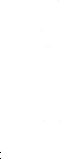
Looking at it from another side, after some given distance, the phase factor is di erent for di erent positions within the pulse profile: It is largest at pulse center and tapers o in the wings. In other words, the pulse acquires a phase modulation known as self-phase modulation (Fig. 9.2). This is a crucial insight for much of the remainder of this discussion, and it will be discussed in more detail below.
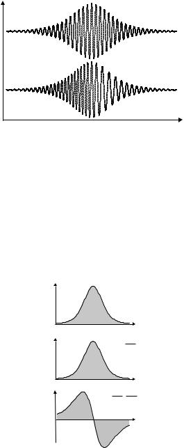
Self-phase modulation may also be interpreted as self-frequency modulation since phase and frequency modulation are closely related. Using the nonlinear phase φnl = γP L, at some position L, the frequency deviation due to nonlin-
earity is
ω = dφnl = γL dP , dt dt
as shown in Fig. 9.3. Self-frequency modulation is frequently called chirp; a self-frequency-modulated pulse is said to be chirped.
9.3.5Dimensionless NLSE
Let us compare the characteristic lengths (we use P0(0) = P0):
Lα = 1/α depends solely on fiber properties.
LNL = 1/γP0 = (cAe )/(n2ω0P0) depends on the fiber (on Ae and n2) and on the signal (ω0 and P0). The signal dependence is only by the instantaneous value, not the temporal profile.
9.3. Nonlinear Wave Equation |
163 |
Field amplitude
Propagation direction
Figure 9.2: Impact of self-phase modulation. Top: Within a light pulse, the optical field oscillates at a certain frequency; the envelope defines the pulse duration. Let such a pulse be launched into a medium where there is selfphase modulation. Bottom: After passing through that medium, phases have shifted. Propagation is maximally slowed down at pulse center; therefore, waves appear pulled apart in the rising slope (right ) whereas they are compressed in the trailing slope (left ).
I(t) |
|
|
|
I(t) = sech2(t ) |
|||
|
|
t |
|
φNL(t ) |
γ L |
|
|
φNL(t) = |
I(t ) |
||
Aeff |
|||
t
Δω(t) |
γ L dI(t) |
Δω(t) = |
|
|
Aeff dt |
|
t |
Figure 9.3: Sketch to explain the connection between self-phase modulation and self-frequency modulation. Top: Let the intensity profile be bell-shaped as shown, e.g., sech2(t). Center : The nonlinear phase follows the intensity profile. Bottom: The instantaneous frequency is given by the temporal derivative of the phase and thus follows the temporal derivative of intensity.

164 |
Chapter 9. Basics of Nonlinearity |
LD = T02/|β2| depends on the fiber (|β2|) and on the signal (T0). This time the signal dependence is by the temporal profile, not the absolute values.
By way of these di erent dependencies, combinations of all kinds are possible according to circumstances. A comparison of the characteristic lengths allows to see at one glance which e ects are relevant. Certainly the e ect represented by the shortest length scale will give the most important contribution.
Consider the case that of the three coe cients in Eq. (9.25), only α = 0 and thus Lα → ∞. This is a case of particular interest, an interplay between dispersion and nonlinearity. It permits, among other things, pulse compression and solitons. Realistically, this situation is obtained whenever LD and LNL are comparable but much shorter than Lα. This is the case when short (e.g., picosecond) light pulses propagate in optical fibers.
Using new variables
|
= |
A |
|||||
U |
√ |
|
|
|
|
||
P0 |
|
||||||
|
|
z |
|||||
ζ |
= |
|
|
(9.31) |
|||
|
|
||||||
|
|
LD |
|||||
τ |
= |
T |
|||||
|
|
|
|
|
|||
T0 |
|||||||
|
|
||||||
we rewrite the wave equation with α = 0 as
i |
∂U |
= |
1 |
sgn β2 |
∂2U |
− |
LD |
|U |2U. |
(9.32) |
∂ζ |
2 |
∂τ 2 |
LNL |
There is a signum function here; this is easily explained by the fact that LD is defined in terms of the absolute value |β2|. The factor LD/LNL can be scaled out by using u = N U :
|
|
|
LD |
|
|
|
|
|
|
. |
|
N = |
|
= |
P0T02 |
γ |
|
(9.33) |
|||||
LNL |
|
||||||||||
|
|
|
|
|
|β2| |
|
|||||
Now the equation takes the form
i |
∂u |
± |
1 |
∂2u |
+ |u|2u = 0. |
|
(9.34) |
|
∂ζ |
2 |
|
∂τ 2 |
|||||
This is the celebrated nonlinear Schr¨odinger equation in its dimensionless form, as it is most often found in literature. The sign corresponds to −sgn β2 and stands for anomalous (+) or normal (−) group velocity dispersion, respectively.
There are two possibilities for this sign. Therefore the reader may well guess at this point that there will be two distinct types, or classes, of solutions. Within each class the numerical values of parameters merely act as scale factors for the solution but do not a ect its functional type. But, of course, there is also the very special case of β2 = 0 which requires a careful analysis of its own. Just because the β2 term in the series expansion, Eq. (4.19), is zero does not at all imply that all the higher-order terms vanish as well. In that case, higher-order dispersion must be taken into account.

9.4. Solutions of the NLSE |
165 |
9.4Solutions of the NLSE
In this section, we study solutions of the nonlinear Schr¨odinger equation (9.34). First of all, there is the trivial solution
u ≡ 0. |
(9.35) |
There is no need to waste time on this one. |
|
9.4.1 Modulational Instability
More interesting is the continuous wave solution
u = √ |
|
eiu0ζ . |
(9.36) |
u0 |
For this solution it is important to check the stability. This can be done by inserting a small perturbation away from the solution in a procedure called linear stability analysis. The solution is stable when the perturbation produces an opposite restoring action so that it decays with time. In the opposite case – when the perturbation keeps growing – the solution is unstable.
The continuous wave solution can be either stable or unstable depending on the sign of dispersion (this is shown, e.g., in Chap. 5 of [17]). For anomalous dispersion perturbations grow. The term modulational instability indicates that perturbations at certain frequencies grow faster than others.1 The growth rate, or instability gain, has a frequency dependence [17]
gω = |β2|ω |
Ω2 − ω2 |
|
|
|
(9.37) |
|||||||||||
with |
4 |
|
|
|
|
|
ˆ |
|
|
|
|
|||||
|
|
|
|
|
|
|
|
|
|
|
|
|
||||
Ω2 = |
|
|
|
|
|
= |
4γP |
, |
|
|
|
|||||
|
|
|
|
|
|
|
|β2| |
|
||||||||
|β2 |
|LNL |
|
|
|
|
|||||||||||
ˆ |
|
|
|
|
|
|
|
|
|
|
|
|
||||
where P denotes the peak value of the power. |
|
|
|
|
|
|||||||||||
The gain maximum is |
|
|
|
|
ˆ |
|
|
|
|
|
|
(9.38) |
||||
|
|
|
|
|
|
|
|
|
|
|
|
|
|
|||
gmax = 2γP |
|
|
|
|
|
|
||||||||||
and occurs at the frequency |
|
|
|
|
|
|
|
|
|
|
|
|
||||
|
|
|
|
|
|
|
|
|
|
|||||||
ωmax = |
1 |
√ |
|
Ω = |
|
2γPˆ |
. |
(9.39) |
||||||||
2 |
||||||||||||||||
|
|
|||||||||||||||
2 |
|
|
|
|
|
|
|
|
|β2| |
|
||||||
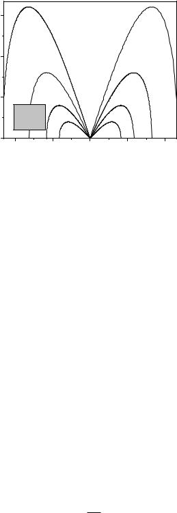
Figure 9.4 shows the spectral profile of this gain.
9.4.2The Fundamental Soliton
The next solution of the nonlinear Schr¨odinger equation exists in the case of anomalous dispersion (for β2 < 0, i.e., on the long wavelength side of the zerodispersion wavelength) and takes the form
u = sech(τ ) eiζ/2. |
(9.40) |
1In hydrodynamics there is the analogous phenomenon under the name of Benjamin–Feir instability [121].
166 |
Chapter 9. Basics of Nonlinearity |
MI gain factor (km–1)
15
4 W
10
2 W
5
|β2|=15 |
|
|
1 W |
|
|
|
|
|
|
γ = 2 |
|
|
0.5 W |
|
|
|
|
|
|
0 |
|
|
|
|
–200 |
–100 |
0 |
100 |
200 |
Frequency difference (GHz)
Figure 9.4: Gain factor of modulational instability. It is assumed that β2 =
2 |
ˆ |
15 ps |
/km and γ = 2/(Wkm). P is given as a parameter. |
The time-dependent part is a hyperbolic secant (or “sech”) function; it therefore describes a bell-shaped pulse. (Some information on sech is gathered in Appendix E). The position-dependent part is an exponential function acting as a phase factor; it rotates through 2π over the distance ζ = 4π. The pulse shape (power profile) is constant since the only dependence on position is in the exponential, see Figs. 9.5, 9.6, and for comparison Fig. 9.7. The pulse shape is also stable in the sense that a certain perturbation away from the precise shape can heal out: a remarkable property which we are going to discuss some more!
This solution is a “solitary” solution in the sense that – in marked contrast to solutions of linear di erential equations – the peak amplitude is fixed; if the solution is multiplied by any constant real factor other than unity, the result is not a solution. From this property derives the name of this solution: it is called a soliton. Indeed this is just one particular representative of a wider class of solitons, and it is more precisely called the fundamental soliton or N = 1 soliton for reasons which we will see shortly.
Fiber solitons are light pulses which do not change their shape during propagation even though at the same time both dispersion and self-phase modulation act on it. It should be more than obvious that pulses with this property must be highly interesting for applications!
When we convert the dimensionless solution back to real-world units, we note: The condition for a fundamental soliton is
LD = LNL N = 1. |
(9.41) |
ˆ |
2 |
By virtue of Eq. (9.33), the peak power of the N = 1 soliton is P1 |
= |β2|/γT0 . |
In other words: All N = 1 soliton share the property that the product of peak power and the square of the pulse duration is a constant, determined solely by fiber parameters:
Pˆ1T02 = |
|β2| |
(9.42) |
|
γ |
|||
|
|