Fiber_Optics_Physics_Technology

window at 1.3 μm and is the first to transmit in a digital format. Its two pairs of fibers, each with a capacity of 280 Mbit/s, allow it to transmit 40,000 telephone channels. The cost per channel is thus dramatically lowered by two orders of magnitude. A steel cladding of the cable is used to provider electrical energy as a supply for the repeaters. At a constant current of 1.6 amperes a voltage of 7,500 Volts is required, the return is through the ocean water. One year later a transpacific cable TPC-3 and a connection between mainland USA and Hawaii, HAW-4, follow in the same technology. These cables form the first generation of fiber-optic intercontinental cables. TAT-8 is decommissioned in 2002.

1991: Fiber-optic cables surpass telephone satellites in terms of number of transmitted calls. 33 million km of fiber have been laid out. Half of it, 16 million km, is in the USA. Europe has 9 million km, the Pacific Rim 8 million km.

1992: The first cable of the second generation, TAT-9, starts in March. The wavelength is now in the third window at 1.55 μm. Advanced components like DFB lasers and APD diodes are used; the transmission format is NRZ. At 565 Mbit/s per fiber in two fiber pairs, 80,000 telephone channels are transmitted simultaneously. The cable is 9,310 km long. It costs 450 million US$ and is owned by a consortium from 35 international telecommunications companies. It links USA and Canada on one side with England, France, and Spain on the other. For Spain, it is the first fiber-optic direct link to the USA; before, they had to be content with TAT-5 with 845 telephone channels. Italy, Greece, Turkey, and Israel are connected via Spain.

In 1992/1993, the same technology is used in the Pacific for TPC-4. The next cables (TAT-10 between USA and Germany/the Netherlands) and TAT-11 are configured in a new topology: Instead of a line between two points a “ring” is used, basically a pair of independent cables between the same two points. The rationale is that if any damage occurs at any position, one can route all data tra c around the damage location. The idea is to ultimately have nets, or webs, that can better survive damage. In view of the enormous data tra c, it is clear that any service interruption immediately leads to considerable financial damage. Like the earlier fibers before, TAT-11 is switched o in 2004.

1994: Unification of Germany has created a new market for telecommunication because in communist Eastern Germany telephones had been available only to a narrow privileged class. Meanwhile in the 1980s, Western Germany had fallen behind other countries in making the transition to fiber optics because the responsible ministry favored copper cables. In the late 1980s this course was reversed, and Western Germany invested heavily in fiber optics. After unification 1990, this situation led to the inspired decision to immediately go for the most advanced technology as the country’s telecommunications infrastructure got an overhaul. Within a few years, the existing 111 lines between both Germanies were replaced with several tens of thousands. In mid-1994, Deutsche Telekom had the world’s most close-meshed fiber-optic network. At a total length of 80,000 km, the fiber network exceeded the highway network. Also, Deutsche Telekom started early to put fibers all the way to the subscriber, an activity which is now described with several new acronyms: FTTH is for fiber to the home,

FTTC for fiber to the curb, and FTTP for fiber to the premises. These acronyms can be wrapped up under FTTx for fiber to the whatever.

1995: The third generation begins with TAT-12; TAT-13 follows in late 1996, and TPC-5 and TPC-6 soon thereafter. Again important technical novelties have been introduced. Dispersion shifted fiber is used; Erbium-doped fiber amplifiers make it possible to increase the distance between repeaters. Now RZ is used as the transmission format. The data rate is 5 Gbit/s equivalent to 1,228,800 telephone channels. Meanwhile, a good fraction of the total tra c is no longer traditional telephone voice communication (“POTS” or plain old telephone service), but also fax and data transmission between computers. Cost per telephone channel has again come down from TAT-8 levels by more than an order of magnitude. TAT-8 through TAT-11 are decommissioned 2002 and 2003. Technically they still work well, but the more recent cables are so much superior that it does not make any business sense to keep them alive. Some of the decommissioned cables have later been used for research purposes.

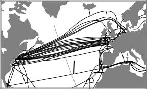
2001: The transatlantic cable TAT-14 takes up service in May. It has been built for 1.5 billion US$ and can handle 640 Gbit/s (corresponding to 8 million telephone calls). In October, a competing consortium opens Flag Atlantic-1 on the same route; this cable has six fiber pairs with a combined capacity of 4.8 Tbit/s. The telecommunications industry thrives on short return-on-investment time and gigantic growth figures. Many competitors join the industry to lay and operate fiber-optic cables (Fig. 11.22). For the

Figure 11.22: Numerous fiber-optic cables crisscross the oceans of the world; on the North Atlantic route there is a particular multitude. The dotted auxiliary line crosses (counting from south to north according to the arrow direction) the cables Columbus-2, Columbus-3, TAT-9, TAT-8, Apollo (southern route), Flag Atlantic 1 (southern route), TAT-14, Flag Atlantic 1 (northern route), TAT-13, Tyco Global Network Transatlantic (southern route), TAT-11, Gemini (southern route), Atlantic Crossing 1 (southern route), TAT-12, Apollo (northern route), Atlantic Crossing 2, PTAT-1, Hibernia (southern route), Gemini (northern route), Tyco Global Network Transatlantic (northern route), TAT10, TAT-14, AC-1 (northern route), Hibernia (northern route), and Cantat-3. In 2005 Tyco sold its Global Network Transatlantic cables to VSNL; they are now called VSNL 2001. For more detail about these cables the reader is referred to [12]. The author has attempted to show all optical cables on this route as of June 2009.

first time in the history of telecommunication, there is an excess capacity: supply surpasses demand. As a consequence the prices come further down, and revenues of all involved parties plummet. There is a string of insolvencies, some of which are quite spectacular (2002: Global Crossing, WorldCom). This is at the same time that the internet bubble bursts, and the two upheavals are related. Euphoria from the late 1990s dissipates very quickly, and recovery to normal business takes several years.

Also in 2001, Lucent Technologies rolls out a new DWDM system called Lambda Extreme for use on long-haul and ultralong-haul segments. It is based on dispersion-managed soliton transmission with Raman amplification, and is specified for 128 × 10 Gbit/s wavelengths (1.28 Tbit/s) up to 4,000 km or 64 × 40 Gbit/s wavelengths (2.56 Tbit/s) up to 1,000 km, at a bit error rate of better than 10−16 [6].

2002: This year heralds the start of commercial soliton transmission systems to carry actual life tra c. Lucent’s Lambda Extreme technology is deployed between Tampa and Miami (both Florida). Existing fiber designed for only 10 Gbit/s and owned by Verizon is used over a distance of 500 km to transmit 100 Gbit/s signals. In Germany, Deutsche Telekom conducts trials over 4,000 km with Lucent’s 128-channel version of Lambda Extreme [14]. While there are several sales of this soliton-based system over the next few years, Lucent does not publicly disclose any details, and available information is spotty.

British equipment manufacturer Marconi Solstis deploys an all-optical network based on solitons which takes up operation at the turn of 2002/2003. This ultralong-haul optical DWDM system, operated by the Australian carrier IP1, consists of a 2,900 km all-optical connection (without signal regeneration) between Perth on the west coast of Australia and Adelaide on the south coast. It uses standard single-mode fiber; solar-powered amplifiers are typically spaced 90 km along the link. It is configured to use 40 out of possible 160 channels of 10 Gbit/s each for later upgrade capability. The system works well in technical terms. Unfortunately, at a time when the telecom industry is forced to release their workforce by the tens of thousands it does not work equally well in business terms, so that it gets decommissioned after only a few years.

Also in 2002, improved fibers are introduced by major fiber manufacturers. Due to increased purity they avoid the OH absorption peak near 1.4 μm so that in e ect the second and third transmission window are merged into one that stretches from ca. 1,280 to 1,625 nm.

2003: The dotcom bubble and ensuing economic woes have haunted the telecom industry for several years, but business is gradually coming back to life. New cables are being installed all the time (e.g., Apollo on the North Atlantic route in 2003), but certainly not at the same hectic pace as before. During the crisis, research is also trimmed back in the companies involved because they cannot generate the revenue that it takes to run large labs. One of the major telecom equipment providers, Lucent Technologies with its famous Bell Laboratories, is sold in 2006 to the French company Alcatel. Two years later, Alcatel-Lucent is pulling out of basic science, material physics, and semiconductor research and will instead

turn its focus on more immediately marketable areas such as networking, high-speed electronics, wireless, nanotechnology, and software.

2007: In March, the record data transmission rate over a single fiber reaches 26 Tbit/s, at a span length of 240 km [52]. At that rate, this entire book could be transmitted in under 1 ms. This is not a soliton system, but it makes use of all the tricks that are there in “linear” systems. It uses 160 WDM channels and polarization multiplexing. For coding, an RZ format and di erential quaternary phase shift keying is used (see below in Sect. 11.4.2); this achieves an impressive 3.2 bits/(s Hz) of spectral e ciency. Distributed Raman amplification balances the losses. Just 5 years earlier, before the introduction of OH peak-free fibers, this signal would have come close to reaching the limit of the available bandwidth.

2009: The major wire-line equipment providers never found back to their strength of the 1990s. The telecom business is now driven in large part by nifty end-user devices like wireless handheld sets loaded with features such as email and Internet access. Meanwhile, in the wake of the US housing bubble another economic recession has arrived. To give just one example, Canada’s Nortel Networks Corporation was worth 250 billion US$ a decade ago, but now initiates bankruptcy proceedings. The global market for telecom services is estimated at 1.7 trillion US$, but an increasing share of this amount goes to wireless operators and handheld providers [67]. It may be anticipated that those of the once big suppliers that remain will see more or less steady, but certainly not stellar business in the years ahead.

Also in 2009, a first commercial 100 Gbit/s system is being deployed and is slated to become operational before the end of the year. It uses dualpolarization QPSK and will be used for rapid exchange of data in the financial industry [8].

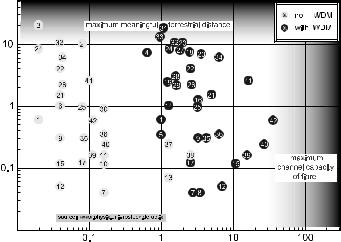
A new record transmission over a single fiber is reported in May: 32 Tbit/s over a distance of 580 km (Fig. 11.23). 320 WDM channels at 25 GHz spacing were used; coding was done in both polarization multiplex and phase shift keying [168].

In assessing the situation today (i.e., summer 2009), one should not forget that large segments of the earth are not yet covered with fiber-optic access. This applies to parts of the Far East, but especially to most of Africa. A first attempt called “Africa One” was planned as a cable forming a ring around that continent; a couple of branches were to tap into countries in the continent’s interior. However, the project was abandoned due to financial problems. Given the sorry state of telecommunication in Africa even today, there seems to be a lot of opportunity there.

11.4.2The Limits to Growth

The tremendous increases in transmission rate over the years became possible after a string of technical improvements such as Erbium-doped fiber amplifiers, dispersion managed fibers, massive wavelength division multiplexing, and the use of nonlinear e ects (solitons, nonlinear chirp). Today, a multitude of data sources is interleaved by TDM to bit streams of 2.5 or 10 Gbit/s, and 40 Gbit/s

Bit rate (Tbit/s)

Figure 11.23: Record experiments for high data rate transmission over a single fiber. The figure does not distinguish between di erent coding formats. For the key to the data points and detailed information see [15], a compilation maintained by Dr. Michael B¨ohm, Rostock University. The figure shows the situation in June 2009.

is now being introduced after years spent learning to live with polarization mode dispersion. Then, several such bit streams are combined by WDM and launched into a fiber. The phrase massive wavelength division multiplex (or with the unavoidable acronym, MDWM) is used when indeed large numbers (on the order of a hundred) channels are used.

Currently the record data rate transmitted over a single fiber stands at 32 Tbit/s. Spectral e ciencies around 0.4 bit/s/Hz are quite normal, but larger values have been obtained as described above.

Since fibers o er a bandwidth of ca. 50 THz, Shannon’s theorem predicts for binary signals a channel capacity of 50 Tbit/s – assuming a spectral e ciency of 1 bit/s/Hz. Obviously the limit is almost reached. It might have been reached already had it not been for the economic crisis which slowed the 200%/year growth before the turn of the millennium to a temporary standstill in the first years of the new millennium.

There are several reasons why the Shannon limit as quoted here needs to be modified somewhat.

1.In contrast to intensity modulation, single sideband amplitude modulation (SSB) or phase modulation with coherent detection (PSK) allow an increase by a factor of 2.

2.An optical fiber supports two polarization modes. This also translates into a potential data rate increase by a factor of 2.

3.Shannon’s theorem holds for a linear channel but the fiber is inherently nonlinear.

And of course one might go beyond binary coding and transmit more than 1 bit/time slot.

Ad 1. In the most recent schemes, often QPSK (quaternary phase shift keying) is used, a format in which the optical phase can assume four di erent values in 90◦ increments. This constitutes a quaternary, rather than binary, coding.

Ad 2. Both polarization modes are not entirely independent from each other; rather, there is some crosstalk between them. This is why it is unlikely that a factor of 2 can be fully reached. In recent experiments, however, alternating wavelength channels are filled with signals of alternating polarization to reduce channel crosstalk; this way they can be placed closer together which improves spectral e ciency. In one case 1.6 bit/s/Hz was obtained [144]. Another case combining polarization multiplex with differential QPSK for a 3.2 bit/(s Hz) e ciency [52] was already mentioned above; also, a similar scheme was used in [168].

Ad 3. Nonlinearity causes stronger channel crosstalk as soon as one attempts to transmit more than 1 bit/time slot. This is because more amplitude levels lead to an increase in average power (the lowest nonzero amplitude level cannot be reduced for reasons of signal-to-noise ratio), and this leads to increased impairment from four-wave mixing. Mitra and Stark [110] found from simulations that an increase is possible only up to 4 bit/s/Hz. With a somewhat di erent approach, J. Tang [154] arrives at similar conclusions. One could alternatively use several phase angles instead of amplitude levels: but angle coding runs into similar problems and does not give a major advantage [71].

As long as a very di erent coding is not found that would avoid the limitations, the limit to growth will be reached in a few years. There are several ideas floated among researchers, but they will have to prove their worth. We will therefore refrain from speculation.

So far it has always been possible to increase the data-handling capacity of the fiber – even legacy fiber! – and not resort to the trivial but costly alternative of laying more fibers. It is always cheaper to upgrade transmitters and detectors as to put new fibers in the ground (or to secure the rights of way for new cables). Surely there must be an ultimate limit to what fibers can do, but it is not yet clear whether we are close or whether smart ideas will buy more time.

In any event, fibers are the most capable medium to guide information: Free space optics through the atmosphere su ers from extra loss in inclement weather conditions and thus from reduced reliability. Nonetheless, it has recently been explored again as a conduit in special niches, like between o ces in upper floors of neighboring high-rise buildings. In outer space laser beams appear to be a very promising conduit for transmission when pointing direction stability issues are solved, but certainly in vacuum which is free from both loss and dispersion much larger bandwidth is possible in principle. Whatever we have learned from fiber optics in terms of light sources, data formats, and receivers will then be of benefit, but fibers themselves will no longer be needed. However, it will be a while before that happens, and here on the ground fibers will stay with us for a very long time.

2.Transmission lines.

3.Displays that translate the transmitted data into a format accessible to human senses, i.e., typically make them visible or audible.

Of course, the scheme also facilitates the keeping of records of relevant data; witness the “flight recorder” which is of central importance after a plane crash.

It has often been taken for granted that for the transmission one uses an electric quantity: most often a voltage, but there is at least one standard where this is a current. The lines are then usually copper cables. The advantage of this approach is that there are innumerably many suppliers, and sensors can be picked from an unfathomable variety of hardware. Also, there is an abundant supply of well-trained engineers and technicians who are knowledgeable about this technology and can use it very e ciently.

Now enter optical fiber. First, one might have the idea of using sensors that do not translate the original data into an electrical format, but rather into some optical format, like a light intensity or wavelength. There is no di culty in converting this to a display because optical formats are easily assessed at the receiver. All it takes is a photodetector, and one is back to a voltage or current that can be displayed in a routine way. Of course, the question is: If one eventually converts to electrical anyway, why bother with optics?

The point is that during transmission, the data are in an optical format. While on its way across the distance, plenty of adverse e ects can act on the transmitted signal. In the case of electric cables, one severe problem is interference from external electromagnetic fields. To avoid such di culty, one usually provides shielding, which in the case of strong external fields is quite involved. Optical fiber, by contrast, is immune to that kind of interference.

There are some other properties of optical fibers that are advantageous in this context. As we saw earlier, they are small and lightweight. The accompanying savings in space and weight can be quite important, e.g., in vehicles, in particular in aircraft or spacecraft. Also, optical fibers withstand extreme temperatures better than electrical cables. They are also more robust in the presence of aggressive chemicals. Finally, fibers provide perfectly separated electrical potentials, a fact that is greatly appreciated, e.g., in petrochemical installations.

We see, one might have benefits from an optical technology. It is good news that a wide variety of optical sensors is available. There is hardly any physical quantity for which no optical sensor exists. New sensors are added all the time for chemical and other quantities, too.

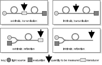
When we look at these fiber-optic sensors, we need to broadly distinguish two classes (Fig. 12.1): There are sensors that are mounted in front of, next to, or in proximity of the fiber, read the quantity under investigation, and launch a corresponding light signal into the fiber. In this case, the fiber is merely the transmission medium and has nothing to do with the acquisition of the original quantity. Such sensors are called extrinsic. In contrast, intrinsic sensors use the fiber itself or part of it directly to read the original quantity. Then the fiber is both sensor and cable at the same time. We will look at examples of both types.

Figure 12.1: Classification of sensor types. In extrinsic sensors (left column), a transducer converts the original quantity to an optical format; in intrinsic sensors (right column) the fiber itself is the transducer. One can also distinguish transmission sensors (top row ) and reflection sensors (bottom row ). The former are simpler in structure because no couplers are required to separate forward and backward traveling light. The latter are more convenient to use, though, because only one end of the fiber needs to be accessible.

12.2Local Measurements

12.2.1Pressure Gauge

The simplest type of an optical pressure gauge is shown schematically in Fig. 12.2. A fiber is placed between two corrugated surfaces; if these are pressed together, the fiber is forced into wiggles and the bending loss increases. By suitable calibration procedure, the amount of pressure can be obtained from the transmission loss. This would be an intrinsic transmission sensor. However, this very simple concept would be susceptible to errors from variation in light source output or any other influences that would e ect the received power.

12.2.2Hydrophone

Quite often fiber-optic sensors make use of the interferometric principle to obtain an impressive sensitivity. The example shown in Fig. 12.3 consists of a Mach– Zehnder interferometer in which a light beam is split into two branches. After passing through similar but independent paths they are recombined again. Any change in the path-length di erence is converted into variations of the resulting power after interference: A change of only half a wavelength provides a 100% variation in the detected signal.

In this example one interferometer arm contains a length of fiber which is encased to insulate it from environmental e ects while the other consists of the