

Fiber_Optics_Physics_Technology
.pdf104 |
|
|
|
|
|
Chapter 7. How to Measure Fiber Characteristics |
|||||
|
|
|
|
|
|
|
|
|
|
|
|
|
|
|
|
|
|
|
|
|
|
|
|
|
|
|
|
|
|
|
|
|
|
|
|
|
|
|
|
|
|
|
|
|
|
|
|
|
|
|
|
|
|
|
|
|
|
|
|
|
|
|
|
|
|
|
|
|
|
|
|
|
|
|
|
|
|
|
|
|
|
|
|
|
|
|
|
|
|
|
|
|
|
|
|
|
|
|
|
|
|
|
|
|
|
|
|
|
|
|
|
|
|
|
|
|
|
|
|
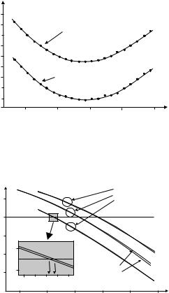
Figure 7.3: Data taken with the setup described in Fig. 7.2. From the propagation time di erentials (top), one finds dispersion through taking the derivative. From [47] with permission.
[162, 92]; then, a minute temperature fluctuation of 0.01◦C creates a change of length by 1 cm in 100 km fiber and gives rise to 50 ps change of propagation time. Therefore procedures are chosen that measure propagation time di erentials between several wavelengths simultaneously. This requires several light sources
I
Change of path difference (mm)
Figure 7.4: Measurement of fiber dispersion in a Mach–Zehnder interferometer. One obtains fringe patterns (interferograms) like the one shown here. Individual fringes are spaced by one half wavelength and are thus too narrow to be resolved on the scale of the figure. In the case shown, a polarization-maintaining fiber was studied; due to its considerable birefringence, there are two clearly distinct groups of fringes.
7.2. Dispersion |
105 |
and has thus higher hardware requirements. On the other hand it provides more direct, uncomplicated data acquisition that reduces manpower requirements. This is a strategy well suited to the needs of fiber manufacturers who always have access to the full-length fiber.
For the other route, it su ces to have a much shorter segment of the fiber, about 1–2 m. The fiber is inserted in one arm of an interferometer; MachZehnder interferometers are the most common arrangement. The reference arm contains either some other fiber with precisely known dispersion or an air path.
Now one can tune (continuously or stepwise) the wavelength of the light source and find, at each wavelength, that path length which maximizes interference contrast. The change of this path length with wavelength leads directly to the fiber’s dispersion (Figs. 7.4, 7.5, and 7.6). Alternatively, one can use
Change of path difference (mm)
1.5
1.0
slow axis
fast axis
1,300 |
1,400 |
1,500 |
1,600 |
1,700 |
Wavelength (nm)
Figure 7.5: Path di erences obtained from the interferogram of Fig. 7.4, shown for both axes of the birefringent fiber. From this, the propagation time di erences are obtained by division with c.
/km) 2 s(p
Dispersion
|
|
|
|
fiber 1 |
|
10 |
|
|
|
fiber 2 |
|
|
|
|
fiber 3 |
|
|
0 |
|
|
|
|
|
–10 |
|
|
|
|
|
1 |
|
|
|
|
|
–20 |
|
|
|
|
|
0 |
|
|
fast axis |
|
|
–30 -1 |
|
|
|
|
|
|
|
slow axis |
|
|
|
1,310 |
1,320 |
1,330 |
|
|
|
–40 |
|
|
|
|
|
1,200 |
1,300 |
1,400 |
1,500 |
1,600 |
1,700 |
Wavelength (nm)
Figure 7.6: Dispersion values β2 obtained from propagation times as in Fig. 7.5. Shown are results for three di erent polarization-maintaining fibers; data for the fast axis (solid ) and the slow axis (dashed ) are nearly on top of each other on this scale. For fiber specimen 3, the range near the zero-dispersion wavelength is shown magnified (inset ): On that scale both curves are clearly separated. Zero-dispersion wavelength for the fast axis here is 1,324 nm and for the slow axis 1,321 nm.
106 |
Chapter 7. How to Measure Fiber Characteristics |
broadband light (white light) and record the interferometric fringe pattern as the path length is scanned; the Fourier transform of that fringe pattern provides the phase information from which dispersion can be calculated. This procedure provides the full wavelength dependence in one go.
7.3Geometry of Fiber Structure
It is also not a trivial task to assess the refractive index profile and the core radius. The direct route is to measure refractive index in an interferometer, but since high spatial resolution is required, a setup involving a microscope is required. One expects refractive index di erences of a few 10−3; for a unique determination, the fiber length must therefore be a few hundred wavelengths; for visible light, this means a fiber length of no more than ca. 100 μm! We conclude that one would have to prepare a thin slice of fiber by polishing which is time-consuming and cumbersome.
There are also methods in which the fiber is illuminated from the side. One first removes the plastic coating, then places the fiber in index-matching gel and shines light through sideways. On a screen one captures a pattern that, in principle, contains the required information. Unfortunately the evaluation is cumbersome again (it requires integral equations) and error-prone. Similarly, one can place the fiber with transverse illumination into an arm of an interferometer. Again one can obtain the information in principle, but only after quite involved evaluation.
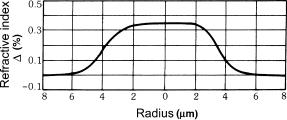
All told, it is a lot easier to assess the internal structure of the fiber before drawing it, i.e., from the preform. Precision is much improved because fine detail of the index profile can be seen clearly while in the finished fiber the same dimensions may be obscured by di raction once they are smaller than one wavelength and thus below the resolution limit (see Fig. 7.7). Details like a nonperfect index step or a central index dip (see Sect. 6.2.1) can be seen much better in the preform (see Figs. 7.8, 7.9, and 7.10).
Figure 7.7: Core profile of a step index fiber, measured from the final fiber. Due to di raction e ects this can show no detail finer than about one wavelength. From [25] with kind permission.
7.3. Geometry of Fiber Structure |
107 |
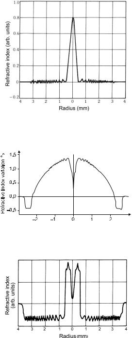
Figure 7.8: Core profile of a triangular fiber, measured from the preform. The preform is much bigger, so much finer detail becomes visible. From [134] with kind permission.
( )


 (
( )
)
Figure 7.9: Core profile of a typical gradient index fiber, measured from the preform. Note the central refractive index dip.
Figure 7.10: Core profile of a double-clad fiber, measured from the preform. Again there is a conspicuous central refractive index dip. From [21] with kind permission.
108 |
Chapter 7. How to Measure Fiber Characteristics |
7.4Geometry of Amplitude Distribution
The distribution of field amplitudes in the fiber is not limited to the core. It also must not be confused with the refractive index profile. The field distribution is wavelength-dependent; roughly speaking, longer wavelengths extend farther into the cladding. In the simplest case of a step index fiber, a relation has been formulated between the mode field radius w (defined as the 1/e point of amplitude), the core radius a, and the V number [96]:
w |
= 0.65 + 1.619 V −3/2 + 2.879 V −6 . |
(7.1) |
|
a |
|||
|
|
Figure 7.11 shows a plot of this relation. The large extent of the mode at long wavelengths (V → 0) is clearly visible, and also the fact that throughout the single-mode regime (V < 2.4048) the mode field radius is larger than the core radius.
10
8 |
|
|
|
|
single- |
multi-mode regime |
|
|
|||||||
|
|
|
|
|
|
||||||||||
|
|
|
|
|
mode |
|
|
||||||||
6 |
|
|
|
|
regime |
|
|
|
|
|
|
|
|
||
|
|
|
|
|
|
|
|
|
|
|
|
|
|
|
|
|
|
|
|
|
|
|
|
|
|
|
|
|
|
|
|
w/a |
|
|
|
|
|
|
|
|
|
|
|
|
|
|
|
|
|
|
|
|
|
|
|
|
|
|
|
|
|
||
4 |
|
|
|
|
|
|
|
|
|
|
|
|
|
|
|
|
|
|
|
|
|
|
|
|
|
|
|
|
|
|
|
2 |
|
|
|
|
|
|
|
|
|
|
|
|
|
|
|
|
|
|
|
|
|
|
|
|
|
|
|
|
|
|
|
|
|
|
|
|
|
|
|
|
|
|
|
|
|
|
|
0 |
|
|
|
|
|
|
|
|
|
|
|
|
|
|
|
|
|
|
|
|
|
|
|
|
|
|
|
|
|
|
|
|
|
|
|
|
|
|
|
|
|
|
|
|
|
|
|
0 |
1 |
2 |
3 |
4 |
5 |
6 |
|||||||||
|
|
|
|
|
|
|
|
V |
|
|
|
|
|
|
|
Figure 7.11: Plot of Eq. (7.1). The mode field radius w is normalized to the core radius a and is plotted as a function of the V number. Throughout the single-mode regime V < 2.4048, w > a holds.
There are several methods to measure the field distribution, and one can distinguish near-field and far-field methods.
7.4.1Near-Field Methods
To correctly identify the field distribution of the guiding mode it is essential that only light from that mode emerges from the fiber end, and that cladding light has died down. Steps to reduce cladding light may therefore be important.
Near-field methods create an image of the mode field distribution in the plane of the fiber face directly. If you now think that you only need to look at the fiber end with a microscope, consider this: We need to distinguish between conventional (or far-field) microscopes and near-field microscopes. Far-field microscopes catch the light di racted out from the object and transform it back
7.4. Geometry of Amplitude Distribution |
109 |
to form an image. They are subject to Abbe’s theory of di raction and do not resolve detail much smaller than a wavelength. This limits the usefulness of the measurement. There are aggravating facts like aberrations and other errors in the imaging; for example, the scale factor is normally a ected by the exact position of the focal plane but enters the final result proportionally so that any uncertainty ends up in the result. Far-field microscope techniques are therefore generally considered not very precise.
A near-field microscope works very di erently. It exploits the fact that a very small aperture, possibly much smaller than the wavelength, still transmits light, if with strong attenuation. On the other hand, this small aperture allows to map out an intensity pattern when it is scanned in the plane perpendicular to the light propagation direction. Then the resolution is not limited by wavelength, but basically by the mechanical resolution of the scanning fixture. Near-field microscopes with atomic resolution have been built.
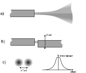
In practice, one uses a second fiber as a probe. The probe is scanned across the fiber tip in very close proximity (less than 10 μm) to map out the power distribution (Fig. 7.12). This is why this is called the transverse o set method. In the limiting case that the probe fiber has a much smaller mode field diameter than the fiber under test, it should be clear that the desired mode structure is obtained directly. Unfortunately this case is unlikely; more typically, both mode fields are of comparable size. Then one obtains the convolution of both distributions; from this the desired shape can be calculated only if the other is well known.
Figure 7.12: Schematic representation of the transverse o set method to measure mode field diameter. (a) The fiber’s exit cone (and the acceptance cone likewise) does not appreciably change its diameter over the first few micrometers. Therefore one can bring two fiber tips closely together. (b) Then one can measure how much power is coupled from one fiber to the other, while the transverse o set is scanned. (c) From mapping out the transmission as a function of position, one can draw conclusions about the mode field diameter.

110 |
Chapter 7. How to Measure Fiber Characteristics |
For typical single-mode fibers and at V numbers not too far from V = 2.4048, the intensity distribution is somewhat similar to a Gaussian:
I(w) = I0 exp(−2(w/w0)2). |
(7.2) |
The mode field radius is taken, by convention, as that radius w at which the field amplitude is down to 1/e ≈ 37% of the central maximum. At this point, the intensity is down by 1/e2 ≈ 13.5% of the maximum. (In old literature sometimes other definitions are found, this can create much confusion.)
The convolution of two Gaussians is a Gaussian again, which makes the Gaussian approximation convenient. The situation is particularly clear when
both fibers have the same mode profile, because they are pieces of the same
√
fiber. Then the convolution has the 2-fold radius of the mode profile of each fiber individually (see Appendix. F), and w0 is obtained by reading the radius where the intensity is down to 1/e of the maximum.
The longitudinal separation of the fibers must be small enough that only the near field, not the divergent part of the exit cone is measured because otherwise one would find systematically too large values.
7.4.2Far-Field Methods
In a very di erent approach, one allows light to exit from the fiber and propagate in free space until the far field is reached. This is the case when the distance z
is at least
λz wλ 2 ,
where w is the mode-field radius (which one tries to determine, but has reasonable guesses about). This condition is easily met already after a few millimeters; in practice, one would prefer a couple of centimeters. At this distance, one can observe the far field, e.g., on a screen. If the distance were increased even more, the pattern on the screen would not change: It would just scale linearly in diameter. It is therefore appropriate to measure positions in the pattern as angles from the fiber tip. The aperture angle of the exit cone is read at the intensity 1/e2 = −8.69 dB referred to the on-axis maximum.
Instead of a screen, one may use a photographic plate or an electronic camera. It is more common, though, to move a single photodetector on segments of circles around the fiber tip as shown in Fig. 7.13 and map out the far-field pattern this way. At large angles with the axis there is only weak intensity, and it is of utmost importance to safeguard against stray light.
If one again applies the Gaussian approximation mentioned in the preceding paragraph, one obtains w0 from the condition
w0 = |
λ |
. |
(7.3) |
|
|||
|
πθ |
|
|
It is much more precise, though, not to make any approximations of that kind. The full information about the field distribution in the fiber is contained in the far-field distribution because the laws of di raction are unique and they are known. A full measurement of the far-field amplitude distribution everywhere on the screen would yield the mode profile unambiguously. (If it were guaranteed that the fiber is circularly symmetric, it would su ce to measure on a diameter
7.4. Geometry of Amplitude Distribution |
111 |
||||||
|
|
|
|
|
|
|
|
|
|
|
|
|
|
|
|
|
|
|
|
|
|
|
|
|
|
|
|
|
|
|
|
|
|
|
|
|
|
|
|
|
|
|
|
|
|
|
|
|
|
|
|
|
|
|
|
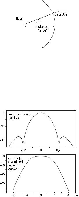
Figure 7.13: Setup for a far-field measurement: In su cient distance from the fiber, a detector is moved on a circular path (or over a spherical surface) centered in the fiber tip. The intensity is recorded as a function of angular position.
instead of the full area.) One would have to apply a Hankel transform, which is a Fourier transform in cylindrical coordinates, using Bessel functions in place of sin and cos.
But there is a catch: Unfortunately one never measures an amplitude distribution, only an intensity distribution (Fig. 7.14). To make matters worse, one also does not measure the entire distribution in a 2π solid angle because that is di cult to do both geometrically and due to the strongly attenuated intensity
Power (dB)
 (
(
 )
)
Power (dB)
 (
( )
)
Figure 7.14: Determination of the mode profile from the far field. Top: Measurement of far-field intensity as a function of angle shows obvious deviations from a Gaussian at large angles. Bottom: The result of a Hankel transform of the far field is the near field, which is the mode profile in the fiber.
112 |
Chapter 7. How to Measure Fiber Characteristics |
at large angles from the axis. Both stray light that finds its way to the detector and the detector’s own noise easily swamp data at large angles.
At large angles to the axis, the intensity goes down so rapidly that cameras cannot easily cope with the required dynamic range. It should be clear that excellent linearity is required throughout the dynamic range. This can certainly not be achieved with conventional photographic means, but electronic cameras are challenged, too. With a good photodiode and possibly with lock-in technology for the weak signals, it is easier to obtain a good dynamic range, limited only by stray light. With due care, 60 dB can be obtained, but even this usually means that at angles larger than 30◦ there is no useful signal.
But back to the amplitudes, rather than intensities: It does not really help to take the square root of all measured intensities because the field amplitude may have zeroes, i.e., nodal lines at which the sign of the amplitude changes. They give rise to dips, or notches, in the far-field profile at certain angles. For conventional step index fibers, the first dip typically occurs at 0.2 rad so that it can be seen only when the dynamic range exceeds 50 dB. The only option is to apply the sign change by hand, but such manipulation should only be performed with utmost care and critical inspection. Sometimes what looks like a null is really only an unresolved minimum. It is precisely the far-field information at large angles that contributes most to the fine structure of the near-field result. As Abbe’s di raction theory asserts, it is the large angle information that carries the high spatial frequency content and is thus responsible for the “sharpness” of the reconstructed near field.
7.5Cuto Wavelength
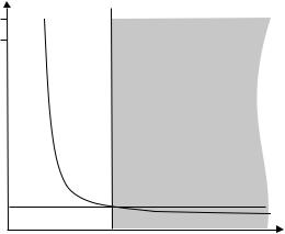
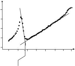
If one determines the mode-field radius as described in the preceding section and repeats the procedure for several di erent wavelengths, one expects to find a trend as shown in Fig. 7.15. There is a characteristic step at the cuto
μm)
Mode (diameter
6
5
1.0 |
1.2 |
1.4 |
1.6 |
Wavelength (μm)
cutoff
Figure 7.15: The mode-field diameter displays a characteristic step at the cuto .
7.5. Cuto Wavelength |
113 |
wavelength because the higher-order mode has a wider field distribution. If one takes this approach to measure the cuto wavelength, one should observe a few subtle points:
We pointed out in the context of bend loss in Sect. 5.2 that the theoretical cuto value at
λcuto = 2πaNA/2.4048 |
(7.4) |
is only found in fibers that are stretched out straight and infinitely long. A definition better adapted to practical requirements therefore identifies the cuto as that wavelength where the loss for the LP11 mode exceeds the loss of the fundamental mode by 20 dB. Strictly speaking, one would have to measure the modes individually to apply this criterion.
For practical use, it is helpful to think this through a little more. For short fibers, the higher-order mode shows up already at longer wavelengths where it is not an allowed mode, but its loss has not diverged yet. On the other hand, bends move the e ective cuto toward shorter wavelengths. If one judiciously selects both fiber length and bend radius, the opposing trends more or less cancel each other out, and one approaches the ideal situation. There is the standard procedure to use a fiber of 2 m length, bent to a loop of 28 cm diameter. Then the cuto is read from the intersection of the asymptotes as shown in Fig. 7.15.
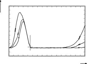
An alternative procedure is a little less involved. One measures the transmitted power as a function of wavelength and repeats with di erent bend radii. Changing the bend radius shifts the loss mostly for the higher-order mode (see Fig. 5.3). From the ratio of spectral transmission with and without bend, one can read the cuto wavelength (Fig. 7.16). The standard procedure is to identify that wavelength at which the transmission di ers by 0.1 dB from that in the plateau above the cuto .
Both this and the previous method occasionally su er from a special complication. Sometimes the characteristic step is not as clear as shown here; instead,
Figure 7.16: Bend loss also shows a characteristic step at the cuto , because higher-order modes are much more sensitive to bending. This allows to find the cuto . Here the additional loss arising from tight fiber loops was used. From [70] with kind permission.