

Fiber_Optics_Physics_Technology
.pdfChapter 1. A Quick Survey |
11 |
What little loss remains in optical fibers is indeed fundamental to fused silica, as detailed in Chap. 5. There have been approaches to reduce loss even further by using other glass types. On theoretical grounds, chalcogenides, fluorides, and halides hold promise to have dramatically lower loss figures than fused silica. Unfortunately, such theoretical considerations never made it into a realization. Production of such fibers is fraught with problems arising from their chemical nature: It is extremely di cult to obtain good purity of a highly reactive substance. Today significant progress in that direction is not anticipated.
Our quick survey would not be complete without mentioning optical nonlinearity. Since the early 1980s, researchers have investigated the nonlinear properties of optical fiber. The term refers to the situation that some optical property of the fiber, such as the refractive index, depends on the intensity of the light wave passing through it. Nonlinearity does not occur in copper cables (at least not to any noticeable degree, anyway), but clearly manifests itself in fibers. This was considered a nuisance for a long time, but today it is increasingly realized that it is precisely the exploitation of nonlinear e ects that allows a new generation of fiber-optic transmission systems, which turns out to be vastly superior to previous technology in its data-carrying capacity. We mention here only in passing the concept of solitons, special light pulses that maintain their shape not in spite of the presence of nonlinearity but due to its presence. In Chaps. 9 and 10, we will discuss nonlinearity and solitons in greater detail.
In some sense, today’s fiber-optic networks have many aspects in common with the telegraph networks of earlier days: either has both attenuation and dispersion; these two represent the biggest practical problems. One can beat attenuation by inserting repeater stations into the fibers at intervals of 50 or 100 km or so. The novelty in fiber optics is that there is nonlinearity, and it causes e ects unknown to electrical systems engineers. Meanwhile, however, the first commercial systems exploiting and embracing nonlinearity and solitons have taken up service, and it can be anticipated that more is yet to come.
We must also point out now that optical telecommunication is by no means the only field of application of fibers. Beyond their enormous data-carrying capacity and great reach, they represent other specific properties that make them attractive for use in data acquisition systems.
One of these properties is the enormous savings in weight, as compared to copper wire. One does not so much realize it by comparing the densities (copper: 8.9 kg/dm3, fused silica: 2.2 kg/dm3) because equal volumes are hardly a relevant basis for comparison. There are protective jackets around both kinds of cable, both for mechanical protection and electrical insulation. These jackets represent the lion’s share of the cable’s mass (bare fiber weighs in at just 30 mg/m). In a realistic comparison between, let us say, fiber-optic cable and coaxial cable for use for transmission in the megahertz regime over a few kilometers, it is a rule of thumb that 1 g of fiber cable replaces 10 kg of electrical cable. (Both reach and data rate of fiber can be scaled up much higher than that of coaxial cable, though.) This represents an immediate advantage where weight limitation is an important requirement: on board of vehicles, ships, aircraft, and spacecraft.
In connection with reduced weight, there is also reduction of space requirement. This is important in cable ducts in inner cities that are crowded already;
12 |
Fiber Optics |
any new installation has to find a way to squeeze in. A fiber-optic cable can replace one or several coaxial cables, upgrade the data rates, and save space at the same time. It is of course better to replace an existing cable in a duct with an upgrade than to install new ducts. Just imagine a work crew digging up Broadway in Manhattan to place more ducts – this is not an option.
As a further distinctive property, fiber-optic cables are immune to electric or magnetic field interference. This is frequently a definitive advantage in industrial installations. Even in close proximity to high-voltage installations, etc., there is no interference picked up by the fiber. This feature sets it apart from electric conductors.
Moreover, glass is chemically quite inert. As long as the fiber’s protective jackets are also made of inert materials, fiber-optic cables can be deployed in chemically hostile environments where metallic parts would quickly corrode. This is attractive for applications in the chemical industry.
And, finally, a fiber-optic cable guarantees a perfect electrical insulation between transmitter and receiver. The same thing can be achieved for electric cables by other means, the so-called optocouplers, but in a manner of speaking, a fiber is an optocoupler stretched long. Di erent fluctuating ground potentials are therefore no longer a concern when subsystems are connected with fiber optics. This is more than a small benefit when there is a potential risk from combustible fumes that one might find, e.g., on oil-drilling rigs. The combination of these properties leads to a fiber-optic sensor technology, which will be discussed in Chap. 12.
Part II
Physical Foundations
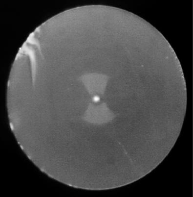
The end of a “bowtie” fiber under the microscope. The fiber’s outside diameter is 125 μm. The light-guiding core is discernible as a small central bright spot. It is surrounded by a bowtie-shaped birefringent zone that gives this fiber type its name. For further information see Sect. 4.6.2 and Fig. 4.18 in particular.

Chapter 2
Treatment with Ray Optics
Calculations in technical optics are often done with a technique called raytracing. This is a treatment of optical systems in the framework of ray optics. It provides a particularly clear, if incomplete, view of the properties of optical systems. Strictly speaking, light propagation needs to be treated by taking the wave nature of light into account. The di erence is that waves give rise to di raction and interference phenomena which are disregarded in ray optics. Whenever the geometrical dimensions of the problem are so small as to become comparable to the wavelength of light, the ray optic treatment breaks down. This is the case in single-mode fibers.
That notwithstanding, we will first present a ray-optical consideration in order to get an idea of the phenomena to be expected. When we then proceed with a wave-optic treatment in Chap. 3, it will become apparent that in fibers the main di erence consists in the fact that the direction of light propagation, which can be any direction in ray optics, is restricted to a discrete set of angles in the full picture.
2.1Waveguiding by Total Internal Reflection
Consider a light ray impinging on some boundary to an optically less-dense medium. Less dense is optics parlance and means “having a lower index of refraction.” At a suitable angle of incidence the ray will be fully reflected, instead of passing through. This process is called total internal reflection and is explained in any textbook on optics (see, e.g., [125, 65, 135]). Total internal reflection plays a role in many contexts: Prisms in binoculars or camera viewfinders use it, and it is the reason why to a diver the water surface appears like a mirror.
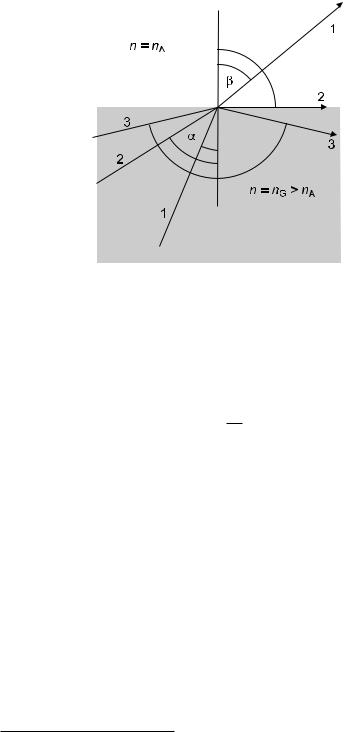
Call the angle of incidence α and the angle of refraction β (Fig. 2.1). At the boundary to the less-dense medium (nA < nG if we think of air and glass), the inequality β > α holds. On the other hand, β cannot exceed 90◦. This becomes clear from an inspection of Snell’s law of refraction
|
sin α |
= |
nA |
|
|
|
|
|
|
|
|
|
sin β |
nG |
|
||
F. Mitschke, Fiber Optics, DOI 10.1007/978-3-642-03703-0 2, |
15 |
||||
c |
|
|
|
||
Springer-Verlag Berlin Heidelberg 2009 |
|
||||
16 |
Chapter 2. Treatment with Ray Optics |
Figure 2.1: On the principle of total internal reflection. The ray coming in from bottom left at angle α strikes the boundary to the less-dense medium and is either refracted (angle β) and transmitted or, if α is too large for that as in case 3, is totally reflected towards the bottom right. Case 2 represents the borderline situation with a grazing angle of the outgoing beam.
when keeping in mind that sin β cannot exceed unity. In that limiting case,
sin αcrit = nA < 1. nG
For even larger angles of incidence, the ray is reflected back into the denser medium nearly without loss. This is the meaning of the term “total internal reflection.”
The same mechanism can also be used to guide light around bends. In 1870 the English scientist John Tyndall (1820–1893) during a session of the Royal Academy demonstrated an experiment which is now part of the standard repertoire of physics course demonstration experiments: A bucket of water is fitted in its lower part on one side with a small hole for the water to spit out, and on the opposing side with a window through which light from a bright lamp illuminates the hole from inside. The water falls in a parabolic curve, and this arc of water guides the light. Some part of the light is scattered o from surface irregularities so that, in a darkened lecture hall, the water column glows in the dark to spectacular e ect (Fig. 2.2).1
The demonstration hinges on the fact that the refractive index of water exceeds that of the air surrounding it. The index of water is about nW = 1.33, while that of air is about nA = 1. Most glasses have indices in the range of nG ≈ 1.4 to 1.8, and therefore the same guiding e ect can be had in strands or rods of glass.
1Tyndall did not invent this himself. The twisted but amusing story leading up to our present-day insights about light-guiding and fibers is reported in [64].

2.2. Step Index Fiber |
17 |
Figure 2.2: Total internal reflection in water lets illuminated fountains glow. Submerged lamps illuminate the fountain from below, and the water column guides it up. This picture was taken in Boca Raton, Florida, USA.
And indeed, fibers exist which consist of nothing but basically a long cylinder of glass or transparent plastic with a diameter of the order of 1 mm. They are used for some special illumination applications, like guiding light into hard-to- reach places inside some apparatus, and everybody has seen those decorative lamps in which a whole bundle of such fibers is combined. Typical optical fibers for data transmission have a somewhat more complex inner structure, though.
2.2Step Index Fiber
A frequently used type of fiber is called step index fiber. Its internal structure is as shown in Fig. 1.3: There is a core with circular cross-section, surrounded by a cladding zone with ring-shaped cross-section. The core consists of a glass with slightly higher refractive index than that of the cladding. Light is therefore guided in the core (but we will need to make this statement more precise in Sect. 3.13). The advantage of this two-layer structure over the simple version is that the fiber surface, i.e., the boundary between cladding and the outside is no longer involved in the light-guiding mechanism. In the event that the fiber surface is soiled or touches other glass, the function is not compromised. The unstructured fiber, in contrast, would su er from enormous loss. Just consider the case that a drop of oil or other liquid comes into contact with the fiber surface: if it had a refractive index comparable to that of the glass, the waveguiding by total internal reflection would break down [158].
18 |
Chapter 2. Treatment with Ray Optics |
|
|
|
|
|
|
|
|
|
|
|
|
|
Figure 2.3: Sketch for calculating total internal reflection.
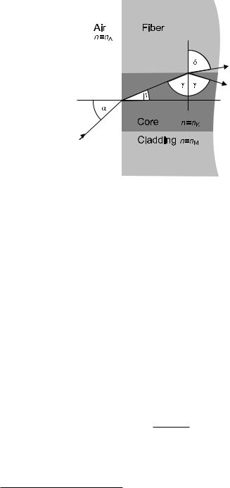
Since the outer surface is not important for the waveguiding in step index fiber, we may simplify its discussion by pretending that the cladding diameter is infinitely wide so that no outside surface exists. Now we can discuss the largest angle with respect to the fiber axis which a ray of light may take and still be guided by the fiber (Fig. 2.3).
Near the fiber end face, we distinguish three refractive indices n, with
nK > nM ≥ nA,
where we used indices A for ambient air, K for core, and M for cladding.2 In the second relation, the equality is valid for unstructured fibers; we will concentrate on step index fibers, though.
We apply Snell’s law:
nA sin α |
= |
nK sin β, |
(2.1) |
nK sin γ |
= |
nM sin δ. |
(2.2) |
When we assume the fiber axis to be perpendicular to the front face, β +γ = π/2 and hence sin β = cos γ. Then
sin β = 1 − sin2 γ. (2.3)
The limiting angle for total internal refraction is defined by
sin δmax = 1 sin γmax = nM/nK. |
(2.4) |
2These indices suggest the German words Kern (core) and Mantel (cladding), respectively. We keep them from the original German edition of this book because the English words core and cladding, as they share the same initial, do not provide a better option. Conveniently, the related English words “kernel” and “mantel” also denote the central part of something and some kind of enclosure, respectively.
2.2. Step Index Fiber |
|
|
|
|
|
|
|
|
19 |
|
Inserting Eq. (2.4) in (2.3) and that in (2.1), we obtain |
|
|
|
|||||||
|
|
|
|
|
|
|
|
|
|
|
nA sin αmax = nK |
1 |
nM2 = nK2 |
|
nM2 . |
(2.5) |
|||||
|
|
2 |
|
|
|
|
|
|
|
|
|
|
− |
|
|
|
− |
|
|
|
|
|
|
n |
|
|
|
|||||
|
|
|
K |
|
|
|
|
|||
We may assume nA = 1 for air. Then the limiting angle αmax for rays to be guided is
αmax = arcsin n2K − n2M.
The argument of arcsin bears a special name: it is called the numerical aperture, often abbreviated as NA:
NA = n2K − n2M.
(The word “aperture” derives from Latin apertus = open and indicates some form of opening. We also find it in “aperitif,” the opening of a meal, and in “overture,” the opening of an opera or a romantic a air. “Numerical” here indicates a dimensionless number.)
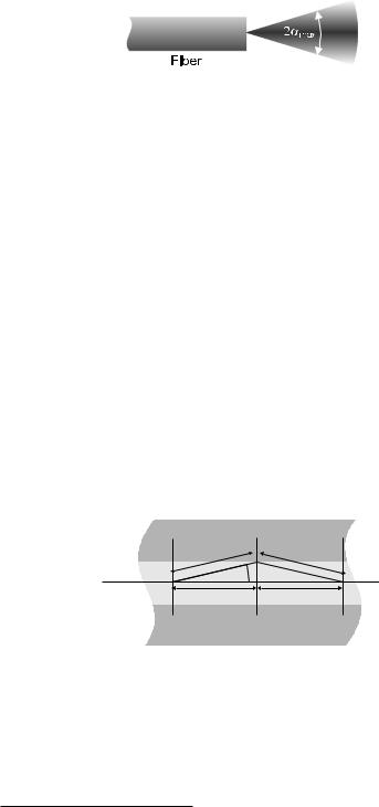
Clearly, the numerical aperture is a measure of the index di erence between core and cladding. The largest acceptance angle for rays hitting the fiber face is given by sin αmax = NA, inside the fiber by sin αmax = NA/nK . Using the fact that in (linear) optics ray paths can be reversed, the acceptance cone at the same time describes the exit cone of light at the other fiber end. In Fig. 2.4, this input/output cone is schematically shown.
We use the opportunity to introduce another frequently used quantity which is also a measure of the index di erence between core and cladding:
|
= |
nK2 − nM2 |
. |
|
(2.6) |
||
|
|
2n2 |
|
||||
|
|
|
K |
|
|||
The conversion between NA and |
is given by |
|
|||||
NA = nK√ |
|
. |
|
|
|||
2Δ |
|
||||||
Usually the index di erence is quite small (a few tenths of 1%) so that |
can |
||||||
be simplified as |
|
|
|
|
|
|
|
≈ |
(nK − nM)(nK + nM) |
|
|||||
nK(nK + nM) |
|
|
|||||
≈ |
nK − nM |
. |
|
||||
nK |
|
||||||
This last relation justifies that |
is called normalized refractive index di erence |
||||||
or normalized index step.
Let us consider typical realistic numbers for single-mode fibers. We assume = 0.3%; with nK = 1.46, this implies NA = 0.11; 0.11 rad indicates an acceptance angle of about ±7◦. Rays hitting the fiber face within a cone of this angle will be guided in the fiber. Rays coming in at steeper angles will leave the core; they propagate in the cladding and move away from the axis. Ultimately they are lost for guiding: The cladding often has more loss than the core, so that part of this light is dissipated. The rest eventually reaches the outside surface where typically a plastic coating is applied for protection; the coating
20 |
Chapter 2. Treatment with Ray Optics |
Figure 2.4: Acceptance and exit cone of a fiber are shown schematically. In reality, the cone is not quite as sharply limited.
has strong optical loss. We conclude that light rays which have left the core once are lost forever.3
In this chapter we have used ray optics. We have seen no reason to assume that within the cone some angle would be preferred over any other one. In the following chapter, a wave-optical treatment will reveal that within the continuum of angles, only a discrete subset is physically possible. These specific angles are related to the so-called modes of the light field in the fiber. The concept of modes is of central importance for the waveguiding properties of fibers and will be studied in detail in the next chapter. However, if many such modes exist, the continuum of angles is approximated again, and our ray-optical approximation is the better justified the more modes there are. In the remainder of our ray-optical treatment we will therefore have multimode fibers in mind.
2.3Modal Dispersion
In this paragraph we will consider the fact that di erent modes, i.e., rays entering the fiber at di erent angles, travel di erent path lengths until they reach the far end of the fiber. Consequently they arrive at di erent times. This scatter of arrival times is known as modal dispersion. Figure 2.5 illustrates the situation.
L’
β
L’
L L
Figure 2.5: Modal dispersion: rays propagating at an angle with the fiber axis travel a longer distance than those remaining parallel to the axis. This leads to di erent arrival times.
In a fiber of length, L, let the path length of a beam propagating at an angle β with the axis be called L . Clearly, L = L/ cos β. Earlier we have seen that sin β cannot be larger than NA/nK. In any event, β 1, and therefore we may
3There is one subtle exception to this otherwise reliable rule: so-called whispering gallery modes will be described in Sect. 7.5.

2.3. Modal Dispersion |
|
|
21 |
approximate sin β ≈ β and cos β ≈ 1 − β2/2. Then we obtain |
|
||
L = L 1 + |
NA2 |
= L (1 + Δ) . |
|
|
|
||
|
2n2 |
|
|
|
K |
|
|
Let us insert the numerical example values from above. With |
= 0.3 % |
||
it follows that L is 3 parts in 1000 longer than L. This implies that the path di erence between the straight and the maximally inclined beam reaches one full wavelength after a distance of 333 wavelengths.
In an interference experiment, one finds a first destructive interference – and hence a mutual cancellation of both rays – after a path di erence of 1/2 wavelength; here, after a distance of 167 wavelengths which corresponds to only a fraction of a millimeter of fiber length. But of course, since both rays propagate at an angle, they do not fully cancel out but rather produce a fringe pattern of parallel bright and dark stripes across their full cross-section. Averaged over that cross-section, the interference e ect cancels out.
Nonetheless, one and the same light signal coupled into the fiber may propagate along di erent paths so that there is a scatter of propagation times often called delay distortion. In the case of short light pulses, this causes an increased duration, i.e., a widening of the pulse. This can go so far that pulses widen to more than their separation; then neighboring pulses spill into each other. When this intersymbol interference happens, the transmitted message is mangled and may be undecipherable.
A rough estimate will su ce to show that this is indeed a serious problem. Let us for simplicity take the velocity of light in the fiber as c/n.4 Then, the propagation time τ for fiber length L in a step index fiber with core index nK is τ = nKL/c. For the ray along the axis, the travel time acquires its minimal value:
τmin = nKL . c
Meanwhile, the ray traveling at the maximal angle takes the longest time:
τmax = nKL (1 + Δ) = τmin(1 + Δ). c
In comparison, the di erence δτ = τmax − τmin is
δτ = |
nKL |
= τmin . |
|
c |
|||
|
|
This shows the simple result that the relative amount of propagation time scatter is given by Δ:
|
|
|
δτ |
|
|
|
|
|
|
= |
. |
|
|
|
|||
|
|
τmin |
|
||
Let us again take |
= 0.3 % as a typical value. In a fiber of 1 km length, the |
||||
arrival times will spread over ca. 15 ns. |
|
||||
This is just a rough estimate, of course: we used approximations and we have neglected that in addition to meridional rays there can also be helical rays
4By doing so, we momentarily ignore the distinction between phase and group velocities.