

Fiber_Optics_Physics_Technology
.pdf9.4. Solutions of the NLSE |
167 |
To illustrate the importance of this product, we note that the energy of the soliton is the time integral of power:
|
|
E1 = +∞ P (t) dt = 2Pˆ1T0. |
(9.43) |
|
|
−∞ |
|
ˆ |
2 |
is something like the time integral of energy, a quantity which in |
|
Then, P1T0 |
|||
classical mechanics is referred to as action. In quantum mechanics, the time integral of the amplitude envelope is called the pulse area [20]; here, action is thus the square of pulse area.
In a given fiber a soliton can have just about any duration, peak power, or energy. However, these quantities always combine such that the action has the same value as given by Eq. (9.42).
If we also insert the relations between T0 and τ (τ = 2ZT0), between β2 and D (D = −(ω/λ)β2), and between n2 and γ (γ = n2(ω0/cAe ) ), then we obtain
Pˆ |
= |
Z |
2 |
λ3 |
|
|D|Ae |
|
1 |
. |
(9.44) |
|
π2c |
n2 |
|
|||||||
1 |
|
|
|
τ 2 |
|
|||||
Here we introduced the numerical constant Z = cosh−1 √2 = 0.8813 . . . for
|
|
|
|
|
|
|
|
¯ |
rather than the peak |
convenience. If we wish to find the average power P1 |
|||||||||
ˆ |
, we write |
|
|
|
|
|
|
|
|
power P1 |
|
|
|
τ 1 |
|
|
|||
|
¯ |
ˆ |
|
|
|
(9.45) |
|||
|
P1 |
= P1 |
· |
|
|
|
|
, |
|
|
Trep Z |
||||||||
where Trep denotes the repetition rate of the experiment. If we finally insert
ˆ |
|
|
|
¯ |
explicitly as a function of easily |
||||
the expression for P1 |
, then we can write P1 |
||||||||
measured quantities: |
|
|
|
λ3|D|Ae |
|
|
1 |
|
|
|
P¯ |
= |
Z |
|
|
. |
(9.46) |
||
|
π2cn2Trep |
|
|||||||
|
1 |
|
τ |
|
|||||
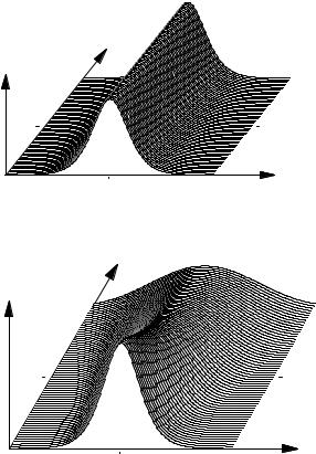
Distance |
Power |
Time |
Figure 9.5: The fundamental soliton in a computer simulation: In spite of dispersion the pulse shape is preserved. Parameters in real-world units: Pulse duration τ = 1 ps, β2 = −18 ps2/km, β3 = 0, γ = 2.5 × 10⁻³/(Wm) and λ = 1.5 μm (see Fig. 4.5). The peak power pertaining to N = 1 is 22.37 W. Shown is the evolution over two soliton periods (56.16 m) in a temporal window of ±5 ps.
168 |
Chapter 9. Basics of Nonlinearity |
Spectral |
Distance |
power |
|
|
Frequency |
Figure 9.6: The spectrum of the fundamental soliton in a computer simulation, using the same parameters as in Fig. 9.5. In spite of nonlinearity the spectral shape is preserved.
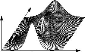
Distance |
Power |
Time |
Figure 9.7: For comparison, here we show the dispersive broadening of a sech2 pulse. Shown is a pulse with an initial duration (FWHM) of 1 ps as it broadens over a propagation distance of 20 m. Of course, the spectrum is preserved in the process – exactly as in Fig. 9.6. The dispersion is β2 = −18 ps2/km and β3 = 0.
The soliton energy is then |
1 |
|
|
|
E1 = |
ˆ |
|
(9.47) |
|
Z |
P1 |
τ. |
Rather than expressing the energy in Joules, it can be interesting to write it as photon number which is found via nphot = E1/(hν) (see Table 9.1).
From these equations we can draw several conclusions: Obviously a soliton can exist for any τ ; it is straightforward to calculate its power. The shorter the duration, the higher the power required to form the soliton. Table 9.1 shows typical orders of magnitude. The table also mentions a characteristic length z0 which is commonly called the soliton period and is given by z0 = (π/2) LD.
Again we convert to real-world units: |
|
|
|
|
|
1 |
π2cτ 2 |
(9.48) |
|||
z0 = |
|
|
|
. |
|
(2Z)2 |
|D|λ2 |
||||
To interpret this quantity, we reinsert the transformation Eq. (9.31) into Eq. (9.40) and find that the phase of the fundamental soliton rotates full circle

9.4. Solutions of the NLSE |
169 |
Table 9.1: Typical orders of magnitude of characteristic soliton parameters. Assumed values are a wavelength of 1.5 μm, a fiber dispersion of β2 = −18 ps2/km corresponding to about D = 15 ps/(nm km), and a nonlinearity coe cient γ = 2.5 × 10⁻³/(Wm) corresponding to n2 = 3 × 10⁻²⁰ m2/W, and Ae ≈ 50 μm2.
ˆ
The table gives the peak power P , the soliton period z0, its energy, and the pho-
ton number, always rounded to three significant digits. In all cases the action W = |β2|/γ = 7.2 × 10⁻²⁴ W s2.
τ |
|
ˆ |
|
|
z0 |
E1 |
nphot |
|
P |
|
|
||||
1 ns |
22.4 μW |
28,100 |
km |
25.4 fJ |
1.92 × 10⁵ |
||
100 ps |
2.24 |
mW |
281 |
km |
254 fJ |
1.92 × 10⁶ |
|
10 ps |
224 |
mW |
2,810 |
m |
2.54 pJ |
1.92 × 10⁷ |
|
1 ps |
22.4 W |
28.1 |
m |
25.4 pJ |
1.92 × 10⁸ |
||
100 fs |
2.24 kW |
281 mm |
254 pJ |
1.92 × 10⁹ |
|||
after a distance
|
|
|
z ! |
|
|
ζ |
= |
|
|
= 4π |
|
|
|
|
|||
|
|
LD |
|
||
z |
= |
4πLD z = 8z0 |
(9.49) |
||
The phase of the soliton rotates with respect to the comoving frame of reference such that it repeats itself after 8z0.
The soliton period z0 plays a central role in the propagation of higher-order solitons, described in Sect. 9.4.5 below. It will therefore turn out to be useful to write the spatial period of the phase, z = 8z0, in terms of physical quantities. The soliton condition Eq. (9.41) gives us two variants:
4πT 2 z = 4πLD = 0
|β2|
= 4πLNL = |
4π |
(9.50) |
|
|
. |
||
ˆ |
|||
|
γP1 |
|
|
In a fundamental soliton, there is a compensation of the linear chirp by dispersion and of the nonlinear chirp by self-phase modulation. This is why fundamental solitons propagate with no change of shape. This makes the fundamental soliton the natural bit of optical data transmission.
In a real fiber, there are some practical complications which are not taken into account in the nonlinear Schr¨odinger equation. In particular, in the presence of a gradual mild energy loss, the shape will not stay constant, but will
170 |
Chapter 9. Basics of Nonlinearity |
readjust according to Eq. (9.42). That is, when a soliton loses some of its energy, it will acquire a somewhat wider pulse shape.
The key here is that the loss occurs gradually (adiabatically): If the power is abruptly reduced (at a splice, say) so that instantly N < 1/2, the soliton is destroyed, and only linear waves carry the remaining energy away. Adiabaticity implies that the loss is negligible over a distance on the order of z0. If in a very long fiber energy is continually drained away from the soliton according to a factor E(z) = E(0) e−αz , the pulse duration T0 will initially increase to accommodate the adiabatic energy loss. This, however, also increases LD = T02/|β2|. Then, the loss per LD (in contrast to the loss per unit of z) keeps growing until, inevitably, at some point the rate of loss exceeds the adiabatic limit. Beyond that point, the soliton is soon destroyed. This process is described in detail in [31]; however, practical systems will always be layed out such that it does not come to this.
9.4.3How to Excite the Fundamental Soliton
What happens when a pulse is launched into a fiber which corresponds exactly to a soliton, except that the peak power is raised or lowered with respect to the soliton peak power? The stable solution of the wave equation is the fundamental soliton, and therefore a soliton will emerge. To accommodate the deviation in power, however, it will acquire a duration and peak power which is di erent from the start values. If the power is reduced, a somewhat longer soliton will be generated (see Fig. 9.8); if it is raised, a shorter soliton (Fig. 9.9). This is the “self-healing property” alluded to above which makes solitons particularly robust entities.
To find the final shape (duration and peak power) of the soliton quantitatively, we consider this: The coe cients of dispersion β2 and nonlinearity γ define that particular value of the action W = |β2|/γ which any soliton in the fiber must have. Even when the launch pulse does not fulfill this condition, the soliton must. Therefore a rearrangement of simultaneously peak power, duration, and energy occurs. Of course there are many ways to vary three parameters
ˆ
at the same time, but they are not independent: P τ = E and Eτ = W . There-
Distance |
Power |
Time |
Figure 9.8: Soliton formation when a pulse with N = 0.8 is launched in a computer simulation. Parameters as in Fig. 9.5 but with N = 0.8 and thus a peak power of 17.9 W.
9.4. Solutions of the NLSE |
171 |
Distance |
Power |
Time |
Figure 9.9: Soliton formation when a pulse with N = 1.2 is launched in a computer simulation. Parameters as in Fig. 9.5 but with N = 1.2 and thus a peak power of 40.27 W.
fore, only a single additional constraint is required to make the rearrangement unique. This constraint comes from energy considerations:
By conservation of energy, certainly the soliton can not have more energy than the launch pulse. But it may have less: then the pulse sheds energy, and the energy of the soliton equals the launch energy minus the energy radiated o .
If the launched pulse happens to precisely match a fundamental soliton (N = 1), the radiated energy Erad is zero. It is also zero for other integer values of N ; larger integers describe higher-order solitons (see Sect. 9.4.5 below). Here, however, we are looking at noninteger N launch conditions. Let us specify
ˆ |
2 |
ˆ |
equivalent to N = 1 + , but we keep | | < 1/2. |
Pstart = (1 + ) |
P1 |
||
The radiated energy is the initial energy minus the energy of the soliton. Using the energy of the N = 1 soliton as a convenient energy unit, this can be written as
Erad = N 2 − (2N − 1).
Then
0.25 : N = 0.5
Erad = 0 : N = 1 ;
0.25 : N = 1.5
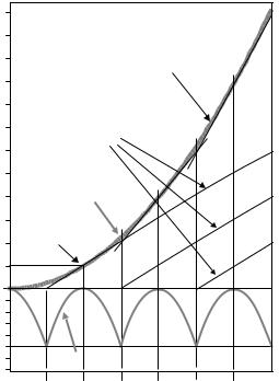
for intermediate values of N one finds values between 0 and 0.25. Clearly, one can specify the energy loss directly. A graphical representation is given in Fig. 9.10:
172 |
Chapter 9. Basics of Nonlinearity |
|
12 |
|
|
|
|
|
|
|
|
10 |
Cumulated soliton energies |
|
|
|
|||
|
|
|
|
|
||||
|
8 |
|
|
|
|
|
|
|
|
|
Soliton energies |
|
|
|
|
|
|
Energy |
6 |
|
|
|
|
|
|
|
4 |
Pulse energy |
|
|
|
|
|
||
|
|
Fundamental |
|
|
|
|
|
|
|
2 |
soliton |
|
|
|
|
|
|
|
0 |
|
|
|
|
|
|
|
|
0.1 |
|
|
|
|
|
|
|
|
0.25 |
Surplus energy (note change of scale) |
|
|
||||
|
|
|
|
|||||
|
0 |
0.5 |
1 |
1.5 |
2 |
2.5 |
3 |
3.5 |
Soliton order
Figure 9.10: Sketch to explain pulse energy and soliton content. If one takes a pulse with fixed duration and increases its energy from zero, beginning at N = 0.5 a soliton is formed. Its energy increases linearly as the pulse energy grows. Beginning at N = 1.5 a second soliton is generated, beginning at N = 2.5 a third, etc. The sum of all soliton energies is a piecewise linear function which runs close to the parabola E N 2 (dashed line) and touches it wherever N is integer. These tangent points are the positions where all energy is invested in solitons. At all noninteger N some part of the energy is not invested into solitons but is radiated o . This part is given by the di erence between the sum of solitonic energies and the parabola; for the sake of clarity, the lower part of the picture shows this di erence on an expanded scale.
Since both action W and energy E are fixed, the remaining parameters are fixed, too:
W |
= |β2|/γ, |
|
(9.51) |
|
E |
= |
Estart − Erad, |
|
(9.52) |
τ |
= |
W/E, |
|
(9.53) |
ˆ |
= |
E/τ. |
|
(9.54) |
P |
|
|||
|
|
ˆ |
2 |
and thus |
This is shown graphically in Fig. 9.11: At constant action, P = (1/τ ) |
|
|||
ˆ |
|
ˆ |
|
|
log P = 2 log(1/τ ). This curve, plotted in a log P – log (1/τ ) diagram, has the
ˆ
slope (d log P )/(d log(1/τ )) = 2. At constant energy, on the other hand, the slope
9.4. Solutions of the NLSE |
173 |
P |
N |
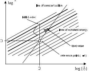
Figure 9.11: Graphical construction of energy and duration of a soliton when
ˆ
the launch condition does not quite fit. In the log(P )-log(1/τ ) diagram, there is a family of curves of constant energy. Also, a particular soliton (fixed τ and
ˆ
P ) is highlighted by a white square. All solitons in this fiber must lie on the curve of constant action (single steeper line). Let the launch condition (hollow circle) have higher energy as required for the N = 1 soliton (the upper of the bold lines). Then, one first calculates the energy loss from Fig. 9.10; then one finds the curve pertaining to the remaining energy (the lower bold line). The intersection of the final energy and the constant action curves gives the soliton’s
ˆ
P and τ .
is unity; shown is a selection from this family of curves. One first identifies the curve of fixed energy pertaining to the launch condition. A second, lower curve is the one where the energy is reduced by just the amount which is radiated o . The final soliton must be on this curve. It must also be on the line designating the soliton action. Therefore, at the intersection of both, we have the final soliton. The coordinates of the intersection point indicate its pulse duration τ
ˆ
and peak power P .
There is an interesting consequence from all this: If one launches a light pulse with N < 1/2 into the fiber, then no soliton will be generated because all the energy is converted to radiation. In a thought experiment, one may consider a fiber with a localized loss (at a splice, say). The condition right after the loss is equivalent to launching a weaker pulse in the fiber. If suddenly N is reduced to values below 1/2 – i.e., when a soliton is suddenly attenuated by at least a factor of 4, it is destroyed: 6 dB localized loss kills a soliton. In stark contrast, a gradual energy loss does not do much harm. This can be seen from the following consideration: If one attenuates first by less than a factor of 4, then allows for unperturbed propagation, a new soliton with lower energy and therefore longer duration will form; some energy will be radiated o and eventually go away by dispersion so that after settling of transients one clearly sees the new, lowerenergy soliton which also has its own N = 1. Then one may attenuate again by less than a factor of 4, and the process repeats. A soliton survives if it is attenuated by a factor of 3 twice, but it dies when it is suddenly attenuated by a factor of 9. For continuously distributed loss, the soliton can survive for a long distance; it will continuously rearrange its width to accommodate its energy level. The long-term decay of a soliton in a fiber has been treated in [31].

174 |
Chapter 9. Basics of Nonlinearity |
9.4.4Collisions of Solitons
The speed of propagation of a soliton in the fiber depends on the optical center frequency due to dispersion. If one launches two solitons with slightly di erent center frequency one shortly after the other, it can happen that both collide. Figure 9.12 shows a computer simulation in which the common “center of mass” of both solitons is the reference frame. During the collision there are some pronounced interference spikes, but afterward both solitons continue their paths unharmed. Both shape and energy of the solitons is maintained; only a phase shift – not visible in the figure – remains. This behavior is reminiscent of that of particles; the name “soliton” is meant to evoke that analogy (think proton, neutron, etc.).
Distance |
Power |
Time |
Figure 9.12: Computer simulation of a soliton collision. Both solitons are intact after the collision.
In optical data transmission, in particular when several wavelength channels are transmitted at the same time (Chap. 11), such collisions can and will happen. The phase shift can have a mild influence there. Other than that it plays an important role in the context of so-called quantum nondemolition measurements in quantum optics (see, e.g., [38]).
9.4.5Higher-Order Solitons
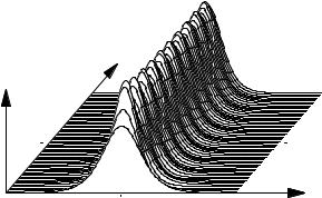
If one keeps increasing the power of the launched pulse beyond the N = 1 point, the soliton gets narrower. But then something remarkable occurs at four times the fundamental soliton power: The pulse goes through di erent shapes as it propagates; this is shown in Fig. 9.13. However, it does so in a periodic fashion, and at certain points along the fiber one finds the sech shape again. (An analytic expression for the complicated breathing shape was found in [136]). This behavior is also reflected in the shape of the power spectrum (see Fig. 9.14). Here we encounter the N = 2 soliton. We ask for its spatial period.
According to Fig. 9.10 at N = 2, there is a superposition of two solitons: One of them has the same energy as the fundamental soliton at N = 1, the other, three times as much. However, both are fundamental solitons: the one with higher power has correspondingly shorter duration. At three times the energy, the pulse width is one third and the peak power nine times that of the lower power soliton.

9.4. Solutions of the NLSE |
175 |
Distance |
Power |
Time |
Figure 9.13: An N = 2 soliton in a computer simulation. Propagation from 0 to 2z0 is shown, i.e., over two oscillation periods.
Spectral |
Distance |
|
|
power |
|
|
Frequency |
Figure 9.14: Spectrum of an N = 2 soliton in a computer simulation, again from 0 to 2z0. Note that the spectrum is broadest where the pulse has the shortest duration (Fig. 9.13).
As both propagate together, their phases evolve at di erent rates due to their di erent power: Eq. (9.50) showed that the phase of the fundamental soliton
ˆ
has completed a full rotation after a distance z = 4πLNL = (4π)/(γP1). Then, for the higher-power soliton, the phase rotates nine times as fast.
As both phases rotate at di erent rates, a beat note is created. The beat pattern will repeat when the di erence between both phases has gone through 2π:
|
9 |
|
|
1 |
|
|
! |
|
φ2 − φ1 = |
|
|
|
ζ − |
|
ζ = 4ζ = 2π, |
||
2 |
|
2 |
||||||
ζ = |
π |
z = |
π |
LD = z0. |
||||
|
2 |
2 |
||||||
As a result we see the true significance of z0: This is the spatial period of the beat note between the constituent fundamental solitons in a higher-order soliton, and hence the distance after which the power profile repeats itself. However, the phase underneath the envelope is repeated only up to a phase factor; it truly repeats for the first time at 8z0 (where one of the constituent solitons has gone through one full cycle, the other through nine).

176 |
Chapter 9. Basics of Nonlinearity |
If the power is increased further beyond the N = 2 case, similar logic can be applied. An N -soliton appears at the N 2-fold power of the N = 1 solitons. All solitons with N > 1 have the property that their pulse shape varies periodically. At integer N the spatial period for the power profile is z0. This disregards phase information; if phase is included, the pattern repeats only after 8z0. Figures 9.15–9.18 show temporal and spectral power profiles of the N = 3 and N = 4 case. The shapes can become quite complex, but they repeat after z0.
Distance |
Power |
Time |
Figure 9.15: An N = 3 soliton in a computer simulation, shown from 0 to 2z0.
Spectral |
Distance |
|
|
power |
|
t |
Frequency |
|
Figure 9.16: Spectrum of an N = 3 soliton in a computer simulation, in correspondence with Fig. 9.15.
9.4.6Dark Solitons
For the case of normal dispersion, a solution of the nonlinear Schr¨odinger equation is given by
u = tanh τ eiζ . |
(9.55) |
When the amplitude profile is described by a tanh(τ ) function, the power or intensity profile must follow tanh2(τ ) = 1 − sech2(τ ). This implies that there is zero intensity at τ = 0 but full intensity far away from the pulse center: a dip in a bright background. Dark solitons are notches in a constantly bright background