Fiber_Optics_Physics_Technology

12.2.3Temperature Measurement

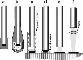
Now we turn to an example of an extrinsic sensor. In the example depicted in Fig. 12.4, the fiber tip is coated with a layer of a thermo-sensitive phosphorescent material commonly called a phosphor (even though no phosphorous is involved). This phosphor, which may actually be magnesium fluorogermanate, is optically excited by a brief flash of light (from an LED) that causes it to emit phosphorescence, i.e., luminescence light with relatively slow exponential decay. The decay time constant is a good metric for the temperature. It is a definite advantage that only ratios of intensities must be assessed to obtain the decay time, but not intensities themselves; any fluctuations due to light source instability, varying connector losses, etc. therefore cancel out. Such fiber-optic temperature gauges are commercially available, and the shape of the sensor can be chosen – depending on intended application – from a variety of several di erent types as shown in Fig. 12.4.

Temperature measurement with fiber-optic sensors have several advantages: The fiber has very small footprint; it has low heat capacity and conductivity and thus does not distort the heat distribution to be measured. Moreover, the sensor is fully dielectric so that measurements are not a ected by the presence

Figure 12.4: Di erent versions of fiber-optic temperature sensors based on the principle of temperature-dependent luminescence decay time. The luminescent material (black ) is deposited on the fiber tip in the standard version shown in (a). The sensor is coated with a protective coating (gray). Variant (b) is optimized for resilience against chemicals and oils; the luminescent material sits in a protective glass ferrule (light gray), which is filled with epoxy (dotted ). In (c), the last 10 cm of the fiber are embedded in a tube made of aluminum oxide ceramics (hatched ). The luminescent substance is supported by a glass bead; an air gap keeps the fiber itself away from temperature extremes. An elastic tip in (d) is meant to provide improved thermal contact with surfaces. (e) and (f ) are versions for noncontact measurement; here the luminescent material is not applied on the fiber but directly on the workpiece. The light emerging from the fiber is reflected and captured again; in the case of extended distance a lens collimates the beam. After [72] with kind permission.

Time (min)

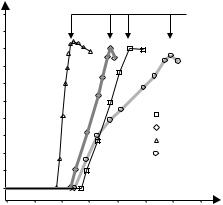
Figure 12.5: Example for an application in which fiber-optic thermometers have a vast advantage: temperature measurement inside a microwave oven during operation. The heating of the components of a meal is shown. Now it has been proven after all that the dessert is almost boiling while the mashed potatoes are still lukewarm! After [72] with kind permission.

of strong electric, magnetic, or electromagnetic fields. Electrical thermometers (thermocouples, etc.) do not share these advantages. Figure 12.5 demonstrates a measurement of the heating process of a processed meal in a microwave oven.

Alternatively, a fiber can also be used for temperature measurement by exploiting its thermo-optic coe cient, which describes the change of refractive index of fiber with temperature changes (there is also a minor contribution from the thermal expansion). The thermo-optic coe cient of fibers is around 30–40 ppm/K [162, 92]. One can use a fiber Fabry–Perot filter or a fiber-Bragg grating and assess the spectral shift of the reflection or transmission maximum. In another variant a Mach–Zehnder arrangement would contain a reference fiber at fixed temperature.

12.2.4Dosimetry

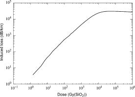
As a final example, we look at a fiber that is subject to ionizing radiation. Dislocations are created in the glass and cause an increased optical loss which can cause a decrease of the transmitted power. The damage is essentially cumulative so that such a fiber can be used as a radiation dosimeter, i.e., an integrating gauge for the cumulative radiation received in a certain amount of time. Fiber-optic dosimeters have a wider linear range than those using other technologies (Fig. 12.6). Moreover the reading tends to be more precise because in any dosimeter, there is some degree of recovery of the dislocations after the irradiation ends. In fiber-optic versions this e ect is less pronounced than in other types, and this makes a di erence when an evaluation takes place only some time later.

Figure 12.6: Calibration curve of a fiber-optic dosimeter. The additional optical loss at λ = 829 nm at room temperature was measured during an irradiation with 60Co at a dose rate of 1.43 Gy(SiO2)/s. The linear range extends across four orders of magnitude. Taken from [69] with kind permision.

12.3Distributed Measurements

A more recent development may push applications of intrinsic sensors far beyond what is conceivable with electric sensors. The crucial point is this: An electric sensor measures at a point – a mathematician might say, on a zerodimensional manifold. A fiber is extended and measures along a line, i.e., one dimensionally. As long as one is only interested in data at certain spots (a zerodimensional manifold), this consideration is moot. However, it is important as soon as one wishes to monitor a higher-dimensional manifold. Examples for one-dimensionally distributed data acquisition are in monitoring the integrity of conduits of all types, including pipelines for oil, gas, or water, or power transmission lines, telephone lines, etc. It may be required to permanently monitor for possible temperature rises, mechanical stress and strain, vibration, etc. It is just not practical to combine many point-like gauges in short distances because the numbers would be excessive. A single fiber can accomplish the same job.

In even higher dimensions it is easy to see: One can lay out a fiber in a zigzag pattern to cover an area. Example: A 2D pressure sensor embedded in the floor can detect whether a person is present in a certain area. This is a useful feature either for ensuring the safety of operators of dangerous machinery or for detecting intruders. Point sensors would have to be distributed in a grid pattern, implying both large numbers and high cost. As one proceeds from line to area to volume, the same logic applies.

Distributed fiber-optic sensors are available, and they provide good spatial resolution to boot! This is accomplished through propagation time e ects. It should be clear how big the advantage is when one can learn in real time not only that an oil pipeline is subject to a worrying mechanical tension somewhere, but when the position of the trouble is precisely located – in some cases, within centimeters. Then, a service crew can be dispatched immediately and fix the problem before major damage occurs.

In such applications, the optical fiber itself is just about the cheapest part. It is therefore not a problem when fibers are buried in concrete when a structure is built. They can then not be replaced later on; therefore they are referred to as “lost fibers.” Nevertheless, as long as their ends (or at least one end) remain accessible, the fiber embedded in a structure can provide important clues about mechanical stresses acting on the structure in real time. This idea has been applied in dams and bridges and has become quite normal now [103]. An early example was Winoosky Dam in Vermont, USA, a dam with turbines providing electrical power [46]. More than 6 km fibers were embedded. Right at the first trial runs of the turbines the fiber-optic sensors showed a conspicuous resonance in the vibration spectrum of one of the turbines: The resonant frequency was at 168 Hz instead of 174 Hz as expected. Given this clue, the turbine’s manufacturer could quickly fix the problem: Due to a defective component the e ciency was 81% rather than 92%! It would have been much more costly to discover that under load conditions during operation, and those savings alone paid for the fibers [2].

Fibers have made inroads into two-dimensional problems: Monitoring stresses on the hull of a ship is now possible in tankers as well as icebreakers. Wind turbines are another obvious field of application. In aircraft, the monitoring of structural integrity of the skin – and the wings in particular – is of the greatest importance. Using a closely knit mesh of fibers, one adds nearly nothing to overall weight but obtains the perfect means of diagnosis. Such a skin with embedded high tech is also known as “smart skin.” Raman scattering types allow temperature monitoring due to temperature-dependent wavelength shifts and find applications in fire detection in tunnels, pipeline monitoring, etc. On the other hand, arrays of fiber-Bragg gratings (mostly for stress and strain detection) seem to be commercially more successful than truly distributed sensing schemes (see Figs. 12.7 and 12.8).

This is again the point where two considerations converge. Large amounts of data as produced by a smart skin need to be transmitted. There is hardly a better medium for this task than optical fiber, an excellent medium for communications. The same on-board fiber network that transmits communications

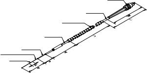
FC/APC-Connector

fiber optical cable Ø3

polymer bending tube Ø5

fiber optical cable Ø3

secondary coating Ø0.9 SM-optical fibre with primary coating Ø0.25

area of Bragg grating

all lengths in mm

Figure 12.7: Package of a commercial fiber-Bragg grating temperature sensor specified for the range −30 to +80◦C with 0.1◦C resolution and 0.5◦C accuracy. With kind permission by Teleg¨artner Ger¨atebau GmbH [1] and by AOS GmbH [3].

Figure 12.8: A commercial fiber-optic strain and temperature sensor designed to be welded directly onto the metal structure to be monitored. This 15 by 40 mm size device is specified to acquire ±2500 μstrain with a resolution of 0.4 μ strain and a temperature of −170 to +150◦C with 0.05◦C resolution. With kind permission of Smart Fibres Limited, Bracknell, UK [4].

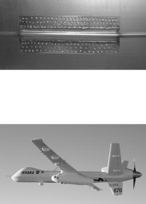
Figure 12.9: NASA’s Ikhana, a modified Predator B unmanned aircraft adapted for civilian research, is being used to test advanced, fiber optic-based sensing technology to monitor structural integrity. Six fibers on the wing’s top surface provide more than 2,000 strain measurements, thus providing full information of the wing shape in real time. They add merely 1 kg of weight and do not appreciably a ect aerodynamics. The data gathered improve safety, but the ultimate goal is to develop active control of wing shape so that the aerodynamics can be adapted to take-o , cruising, and landing. Such capability could dramatically improve e ciency and performance. From [5].

(and is in place anyway) can double to transmit information on mechanical stress, temperature extremes, etc. In the narrower sense of the word this, too, is communication except it is not humans like captain and flight engineer who are doing the communicating, but rather the engine, the wing, and the computer. This approach is used a lot in military craft (Fig. 12.9); while details are typically classified it is a safe bet to assume that all recent constructions of aircraft, ships, and submarines are equipped with a lot of fiber.

Fault tolerance refers to to the ability of equipment to keep working even when part of it is damaged. This is an important requirement everywhere, and in combat aircraft it is absolutely vital. As long as all on-board components are linked through a web-like structure (rather than linear connections), some local damage will result not in an interruption of data flow, but merely in its rerouting.

This is a strategy well known to power utility companies and telephone service providers alike, and it applies to on-board fiber-optic networks, too.

The paradigm of a web structure is the internet which, as is well known, was designed with the idea in mind that it should be nearly indestructible. What cannot be killed even by a nuclear blast is obviously quite robust. Some crooks exploit this robustness by sending us zillions of spam messages or trading in unsavory material, all the while relying on the notion that they are almost unstoppable. This activity is detestable, but it does illustrate the point.

12.4The Status Today

These days structures such as dams, bridges, tunnels, mines, storage tanks, and towers are more and more often equipped with sensors, and fiber-optic types are used increasingly and command an increasing share of the total sensor market. The most frequently used types are based on fiber-Bragg gratings, Raman and Brillouin scattering, and mechanical or thermal length variation.

Fiber-optic sensors are always in competition with existing technology, and must assure a definite advantage before they are adopted. There is the di - culty that on one hand scientists working in research labs are fully prepared to respectfully treat novel technology with care, but that on the other hand in the environment of a major construction site the hard hat-wearing crowd has little patience for the fragility of delicate fibers. If one embeds a fiber in concrete, one should take great care not to break the fiber end at the place where it sticks out of the concrete: If it is broken, it may be useless (and is indeed a “lost fiber”!).

Nonetheless, fiber-optic sensors are big business now: The market for fiberoptic sensors in the USA alone in 2007 was 235 million US$ (170 million for intrinsic, 65 million for extrinsic sensors). At about 30% annual growth, this figure is expected to climb to 400 million US$ in 2009 and 1.6 billion US$ in 2014 [7]. In the Asia-Pacific area the market grows even more rapidly and is expected to reach 190 million US$ in 2009. Defense, aerospace, telecom, and automotive industries are the major users.

Part VI

Appendices

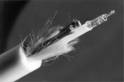
Beyond the fiber itself, a fiber-optic cable contains a complex structure of mechanical elements for protection against abrasion and stress. The picture shows the tube that contains the fiber; not visible is the gel filling. Further outside there are strands of Kevlar fiber acting as stress members. Kevlar is a resilient fibrous material from which, among other things, bulletproof vests are made.

Appendix A

Decibel Units

The measurement units of “decibels” are in widespread use in electrical engineering; both physicists and engineers are expected to use them proficiently. They constitute a logarithmic measure useful for gain factors, attenuation factors, etc. The advantage of using a logarithmic measure is that in a transmission chain, there are many elements concatenated, and each has its own gain or attenuation. To obtain the total, addition of decibel values is much more convenient than multiplication of the individual factors.

A.1 Definition

One decibel is the tenth part of 1 B. The name refers to Alexander Graham Bell; for historic reasons his name is truncated to “Bel.” One Bel designates a ratio of 10:1 between two quantities which have the dimension of a power. Let us call them P1 and P0:

δ[Bel] = log10 P1 . P0

It is also common to use this definition for quantities that are proportional to a power, such as energy, work, energy density, or intensity (power per area). Of course, both quantities involved must be of the same type so that the argument of the logarithm is dimensionless.

In contrast to standard practice in the SI system of units, neither the unit Bel itself nor its combination with prefixes such as milliand microis used. The decibel is the only form in use, and it is abbreviated as dB. In fact, one would rather speak of one hundredth of a decibel than a millibel. A decibel is defined as the tenth part of a Bel, so that

P1

δ[dB] = 10 log10 P0 .

For example, inserting the output power of some amplifier as P1 and its input power as P0, δ[dB] is the gain factor. Negative gain factors imply attenuation.

It is prudent to remember a few selected numbers: 10 dB imply a factor of 10, 20 dB a factor of 100. 3 dB pretty closely corresponds to a factor of 2, and correspondingly, 6 dB to a factor of 4.

c Springer-Verlag Berlin Heidelberg 2009

A.2 Absolute Values

Up to now we described the use of the dB as a relative unit. It can also be used for absolute values when a standardized reference value for P0 is agreed upon. Most frequently, this is the value of 1 mW. Whenever power is measured with reference to 1 mW, the letter “m” is appended to the dB to produce dBm:

P δ[dBm] = 10 log10 1 mW .

For example, the maximum output power of amplifiers is frequently quoted in dBm. Thus, 40 dBm are a fancy way to say 10 W.

Another variant of using dB units for absolute values is in widespread use: dBμV implies dB referred to a reference voltage of one microvolt.

Carried away by the convenience of the notation, some authors use dB for just about all kinds of quantities. There have been sightings of, e.g., the ratio of two resistances in dB. This author strongly recommends against such practice.

A.3 Possible Irritations

When using decibel units, novices frequently get confused in either one of two circumstances.

Amplitude Ratios

The first source of confusion is that decibel is not always used for powers. In electrical engineering in particular, measurement typically yields not power directly, but rather a voltage U or a current I. As a consequence, when providing a gain factor of some device, one needs to specify whether it is a voltage gain, a current gain, or a power gain factor. This distinction disappears when decibel units are used.

According to Ohm’s law and assuming a standard load resistance R,

P = U I = U 2 .

R

Similarly, in optics, the power of a light signal is proportional to the square of the electrical field amplitude. Again, one needs to specify whether the amplification/attenuation is referred to the field amplitude or to the power.

Since

decibels can be used without conflict with the above definition when

A1

δ[dB] = 20 log10 A0

is observed. Here A denotes an “amplitude type” quantity such as voltage and field strength, which is proportional to the square root of a “power type” quantity as described above.