

Fiber_Optics_Physics_Technology
.pdfAppendix E
Relations for Secans
Hyperbolicus
The function Secans Hyperbolicus (hyperbolic secant) is defined as
2 sech(x) = ex + e−x .
For convenience we introduce a numerical factor
Z = |
cosh−1(√ |
|
|
|
≈ 0.881373587, |
|
2) |
||||||
2Z = |
cosh−1(3) |
|
||||
= |
√ |
|
|
≈ 1.762747174. |
||
ln(3 + 8) |
||||||
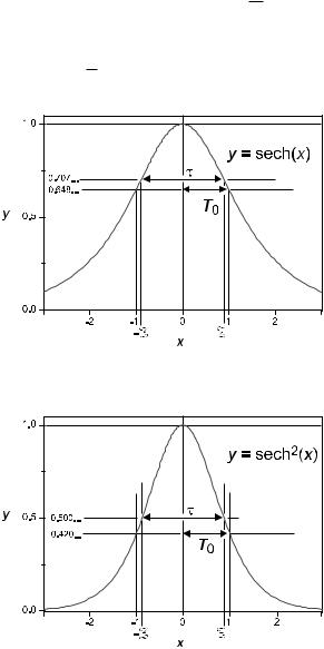
cosh−1 refers to the inverse function arcosh, not the reciprocal of the function. One finds the following special values (Fig. E.1):
sech(0) |
= |
1, |
|
|
||
sech(1) ≈ 0.6480542737, |
||||||
sech(2) |
≈ |
0.2658022288, |
||||
sech(Z) |
= |
1 |
√ |
|
|
|
|
|
2. |
||||
2 |
||||||
|
|
|
|
ˆ |
||
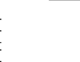
A light pulse with envelope U (t) = U sech(t/T0) has the power profile P (t) = |
||||||
ˆ |
2 |
(t/T0). The following special values hold (Fig. E.2): |
||||
P sech |
|
|||||
|
|
sech2(1) |
≈ |
0.4199743416 |
||
|
|
sech2(Z) |
= |
1 |
. |
|
|
|
|
2 |
|||
The pulse duration, taken as the full width at half-maximum (FWHM), is
τ = 2ZT0. |
|
F. Mitschke, Fiber Optics, DOI 10.1007/978-3-642-03703-0 17, |
273 |
c |
|
Springer-Verlag Berlin Heidelberg 2009 |
|
274 |
Appendix E. Relations for Secans Hyperbolicus |
The pulse energy is
|
|
∞ |
∞ |
|
t dt |
E |
= |
|
P (t) dt = Pˆ |
sech2 |
|
|
|
−∞ |
−∞ |
|
T0 |
|
|
|
|
||
|
|
ˆ |
|
|
|
|
= 2P T0 |
|
|
||
|
= |
1 ˆ |
|
|
|
|
Z P τ. |
|
|
||
|
|
Figure E.1: y = sech(x). |
|||
Figure E.2: y = sech2(x). |

Appendix F
Autocorrelation
Measurement
F.1 Measurement of Ultrashort Processes
It would be a straightforward task to measure duration and shape of picosecond or femtosecond pulses if detectors (and oscilloscopes) with temporal resolution better than the pulse duration would exist.
However, the fastest photodiodes are restricted to temporal resolutions of several picoseconds. A dramatic advance of technology is not anticipated, because the finite mobility of charge carriers themselves inside the solid-state detectors defines the limitation.
For this reason, an entirely di erent method is used for temporal measurements on ultrashort time scales. The central idea is charming: The pulse to be measured is referenced to itself. The technique is known as autocorrelation measurement. It does indeed work – the price to pay is that one does not obtain the full unambiguous information about the pulse shape. To understand the principle, let us first briefly discuss the mathematical concept of the autocorrelation function, without getting too formal.
F.1.1 Correlation
The word “correlation” describes a similarity. If A does something and B does the same at the same time, then the actions of A and B are correlated. If B consistently does the opposite of what A does, then they are anticorrelated. If B acts independently of A, both are uncorrelated.
Speaking more specifically, we will compare two real functions of time, f (t) and g(t). How can we establish a similarity?
First, we take the product of both functions, f (t)×g(t). It should be obvious that this product is non-negative when both functions have the same algebraic sign (no matter which one) at all times – whenever one changes sign, so does the other. On the other hand, the product is negative whenever both functions have opposite sign (again, no matter which function has which sign).
In the event that f (t) and g(t) are, say, independent random functions, either will change sign at random times that usually do not coincide with the moments
F. Mitschke, Fiber Optics, DOI 10.1007/978-3-642-03703-0 18, |
275 |
c Springer-Verlag Berlin Heidelberg 2009
276 |
Appendix F. Autocorrelation Measurement |
at which the other changes sign. The product, then, will be positive at some times, negative at others – and in the long run, either possibility will occur about half of the time. On average the product is zero.
This brings us to the correlation which is the long-term average of the product:
+∞
corr = |
f (t)g(t) dt. |
−∞
For uncorrelated functions this quantity will tend to zero.
What happens if the functions are related? The strongest possible correlation of f (t) and g(t) occurs when both are identical (up to a scale factor), or f (t) = ag(t) with a some positive real constant. In that case, corr will take its (positive) maximum value. If, on the other hand, f (t) = −ag(t), corr takes the same value but with a negative sign. This constitutes the strongest possible anticorrelation.
F.1.2 Autocorrelation
For those trained in Latin and Greek, the word “autocorrelation” is immediately clear: it describes a correlation of something with itself. The autocorrelation function is the temporal average of the product of two functions, which are identical except for a temporal shift τ :
+∞
autocorr(τ ) = |
f (t)f (t + τ ) dt. |
−∞
It is convenient, and customary, to normalize this expression to its maximum possible value, which occurs, as argued above, for τ = 0:
|
+∞ f (t)f (t + τ ) dt |
||
ACF(τ ) = |
−∞ |
|
. |
|
+∞ |
2 |
dt |
|
−∞ f (t) |
|
|
ACF(τ ) has the following properties:
ACF(0) = 1 for any function f (t) (which is not zero everywhere); this is due to the normalization.
−1 ≤ ACF(t) ≤ +1 for all t and any function; the case ACF (t) > 1 is impossible for all t.
ACF(T ) = ACF(−T ): ACF is symmetric.
If f (t) = const., then ACF(t) = 1 for all t, independent of the value of the constant (disregarding the case of zero).
If f (t) = f (t + T ), then ACF(T ) = 1: Periodic functions have a periodic autocorrelation function with the same period. Phase is irrelevant, though.
To develop a feeling for this, consider a few selected functions.
Sine function. If f (t) = A sin(ωt + ϕ), then ACF(τ ) = cos(ωt). This is independent of ϕ. Thus, it is also true for ϕ = π/2, that is, for cosine instead of sine.

F.1. Measurement of Ultrashort Processes |
277 |
Noise. ACF(0) = 1 is true for any function; on the other hand, we noted above that for a random signal, ACF(τ ) = 0. There is no contradiction. At
τ= 0, ACF of noise is equal to 1 and then drops very rapidly to zero as
τgrows. The range of τ over which ACF decays and is still di erent from zero indicates the correlation time of the signal.
The inverse of the correlation time is the bandwidth of the noise; there is no such thing in physics as noise with infinite bandwidth or zero correlation time. Nonetheless that limiting case is important conceptually and is studied by theorists due to its nice mathematical properties. It comes by the name of δ-correlated white noise. Any physical noise has a correlation time that is di erent from zero because nothing in nature ever acts infinitely fast. White noise with infinite bandwidth violates the law of energy conservation.
Gaussian. A signal with a temporal variation according to a Gaussian (a Gaus-
sian pulse) has an autocorrelation function that is Gaussian again, but is
√
wider by a factor of 2. We encountered the spatial case in Sect. 7.4.1: Measurement of a mode profile in the near field by the transverse o set method yields the autocorrelation function of the mode profile. As long
as one can justifiably approximate it as a Gaussian, one can take the mea-
√
sured radius and simply divide by 2 to obtain the correct modal radius.
F.1.3 Autocorrelation Measurements
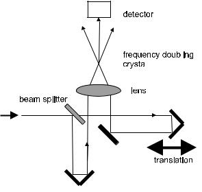
Let us return to our task to measure the duration of ultrashort optical pulses. The procedure involving the autocorrelation function is now easy to understand. In the setup of an autocorrelator, the light beam carrying the pulses is first split at a partially reflecting mirror with reflectivity R = 50%. Thus, there are two paths; on each there is one replica of the pulses to be measured. Both replicas are recombined in a nonlinear crystal. The crystal is chosen such that it can generate the second harmonic of the light (aχ(2) e ect; compare Eq. (3.18)). In this case there always is a term containing the product of two electrical fields. Each partial beam by itself creates such a product of its field with itself, i.e., |E1|2 and |E2|2; of more interest for us is the combination term of E1E2, which is also generated. (In a popular variant called background-free autocorrelation, these three contributions can be geometrically separated and only the combination term is used.)
Finally, a temporal integration is performed. In practice, one does not need to push the integration limits to ±∞; it fully su ces when the integration interval is much longer than the pulse duration. Ironically, a slow photodetector is not only good enough here: it is actually required to be slow!
Both replicas of the incoming beam travel similar, but not necessarily equal, path lengths before they are recombined at the focal point of a lens, which is inside the nonlinear crystal (Fig. F.1). By fine-tuning the path-length di erence, one can arrange that both replicas arrive simultaneously so that a maximum combination product term is generated and registered on the detector.
The measurement is performed in the following way: The path di erence is scanned while the detector signal is monitored. Typically one provides the path di erence information to the horizontal input of an oscilloscope, and the detector signal to the vertical input. As the path di erence is varied, the pulse profile
278 |
Appendix F. Autocorrelation Measurement |
|||||
|
|
|
|
|
|
|
|
|
|
|
|
|
|
|
|
|
|
|
|
|
|
|
|
|
|
|
|
|
|
|
|
|
|
|
|
|
|
|
|
|
|
Figure F.1: Sketch of an optical autocorrelator setup. Two replicas of the pulse stream to be measured arrive at a frequency-doubling crystal through di erent paths. Only if both arrive at the same time can there be appreciable power in the combination product which is monitored by the detector. By variation of the path-length di erence, one can map out the temporal pulse shape.
(or more precisely, its autocorrelation function) is mapped out and appears as a trace on the oscilloscope screen. If this is done at a repetition rate of at least 30 Hz, the eye perceives a flicker-free representation of the pulse shape.
F.1.4 A Catalogue of Autocorrelation Shapes
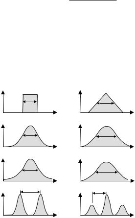
Since it is not the pulse shape directly which is measured, there is always the question of finding the pulse shape that corresponds to the measured autocorrelation function. This is not a unique relation, but in many cases one has some extra information to reduce the ambiguity and gets away with it. We list the relation in Table F.1, and in Fig. F.2 by way of symbolic schematic representations.
It is important to note the following facts: Autocorrelation measurements allow to assess pulse durations down into the few-femtosecond regime; it is conceivable that this can be pushed even further. This exceeds the temporal resolution of direct detection by several orders of magnitude.
On the other hand, autocorrelation measurement do not yield the pulse shape directly. The pulse shape cannot be uniquely reconstructed from the autocorrelation function. (The other way around it would work; alas, that is of little help.) In particular, phase information about the pulse (such as, the existence of a chirp) is lost.
As a consequence, an ambiguous determination of the pulse shape implies an ambiguity in the pulse duration. Absent a better solution, one typically makes educated guesses about the pulse shape based on independent information, then
F.1. Measurement of Ultrashort Processes |
279 |
Table F.1: Table of some selected pulse shapes and the corresponding autocorrelation functions.
Pulse shape |
Corresponding autocorrelation |
||||
|
|
|
|
|
|
Rectangular , width ±1 |
Triangular, width at pedestal ±2 |
||||
Gaussian, width T |
|
√ |
|
|
|
Gaussian, width 2 T |
|||||
sech2(t) |
3 |
t cosh(t) − sinh(t) |
|
||
sinh3(t) |
|||||
|
|
||||
Two equal pulses separated by T |
Three-pronged fork. Prongs separated |
||||
|
by T . Center component is twice as |
||||
|
high as o -center components. Width |
||||
|
of components: ACF of original pulses |
||||
|
|
|
|
|
|
T |
rectangular |
|
|
triangular |
|
|
|
|
|
|
t |
|
T |
τ |
|
|
|
||
T |
Gaussian |
|
|
Gaussian |
|
|
|
|
|
|
t |
1,414 T |
τ |
|
|
|
|
||
|
sech2 |
|
|
|
T |
|
|
|
|
|
t |
1,543 T |
τ |
|
|
|
|
||
T |
pulse pair |
T |
"trident" |
|
|
t |
|
|
τ |
Figure F.2: Schematic survey of autocorrelation signals for di erent pulse shapes. The ACF of a sech2 pulse is given in Table F.1. A pulse pair is represented by a “three-pronged fork”; the center peak is twice as high as the o -center peaks.
280 |
Appendix F. Autocorrelation Measurement |
calculates the pulse width based on that. This is certainly less than exact science. There are more involved procedures giving more detailed information (see, e.g., [157]), but they are not always available. However, as long as the procedures used are stated clearly (like, the width is quoted as “FWHM assuming a Gaussian shape” or so), this is acceptable, and indeed widespread practice. On the other hand, one should not attribute a precision to the widths thus determined, which is not warranted.
282 |
Bibliography |
[13]www.ofsoptics.com/simages/pdfs/fiber/brochure/
AllWave1170305web.pdf
[14]www.opticalkeyhole.com/eventtext.asp?ID=23702&pd=3/20/
2002&bhcp=1
[15]www.physik.uni-rostock.de/optik/en/dm_referenzen_en.html. This website identifies all data points in Fig. 11.23.
[16]Aeschylus, Agamemnon, in: Aeschylus, II, Oresteia: Agamemnon. Libation-Bearers. Eumenides, edited and translated by Alan H. Sommerstein, Harvard University Press, Cambridge, MA (2009)
[17]G. P. Agrawal, Nonlinear Fiber Optics, 4th ed., Elsevier Academic Press, Amsterdam (2007)
[18]G. P. Agrawal, Fiber-Optic Communication Systems, John Wiley & Sons, New York (1992)
[19]N. N. Akhmediev, A. Ankiewicz, Solitons. Nonlinear Pulses and Beams, Chapman & Hall, London (1997)
[20]L. Allen, J. H. Eberly, Optical Resonance and Two-Level Atoms, John Wiley & Sons, New York (1975), Reprint by Dover Publications (1987)
[21]W. T. Anderson et al., Thermally Induced Refractive-Index Changes in a Single-Mode Optical-Fiber Preform, in Proc. Optical Fiber Conference, Optical Society of America, Washington, DC (1984)
[22]E. E. Basch (Hrsg.), Optical-Fiber Transmission, Howard W. Sams & Co., Indianapolis, IN (1987)
[23]P. C. Becker, N. A. Olsson, J. R. Simpson, Erbium-Doped Fiber Amplifiers: Fundamentals and Technology, Academic Press, London (1999)
[24]P.-A. B´elanger, Optical Fiber Theory, World Scientific, Singapore (1993)
[25]G. E. Berkey, Single-Mode Fibers by the OVD Process, in Proceedings of the Optical Fiber Conference, Optical Society of America, Washington, DC (1982)
[26]K. J. Blow, N. J. Doran, Average Soliton Dynamics and the Operation of Soliton Systems with Lumped Amplifiers, Photonics Technology Letters 3, 369 (1991)
[27]R. D. Birch, D. N. Payne, M. P. Varnham, Fabrication of Polarizationmaintaining Fibers Using Gas-Phase Etching, Electronics Letters 18, 1036–1038 (1982)
[28]T. A. Birks, J. C. Knight, P. J. St. Russell, Endlessly Single-Mode Photonic Crystal Fiber, Optics. Letters 22, 961 (1997)
[29]A. Bjarklev, J. Broeng, A. Sanchez Bjarklev, Photonic Crystal Fibers, Kluwer Academic Publishers, Dordrecht (2003)