

Fiber_Optics_Physics_Technology
.pdf8.10. Optical Receivers |
145 |
device shown has a piece of fiber (the “pigtail”) connected to the chip by the manufacturer. Coupling the light of laser diodes into single-mode fibers requires precision; it rarely exceeds 50% in spite of all serious attempts. Therefore it is a great simplification for the end user when this critical step has already been taken care of by the manufacturer.
8.9.4Fiber Lasers
A fiber laser is created when a fiber amplifier is inserted in an optical resonator [40]. The optical feedback provided by the resonator allows a light field (initially starting from spontaneous emission) to build upon itself until saturation e ects arrest further growth: This describes a laser. The energy supply (pump source) must be provided by optical means and is therefore more complex than for laser diodes. On the other hand, fiber lasers are perfectly suited to coupling their light into a fiber: All it takes is a splice. Transverse or lateral modes cannot arise, but the longitudinal mode spectrum has a particularly high number of modes. This is due to the long resonator length and the often very wide gain bandwidth, but is not a disadvantage when modelocked operation is required. A big disadvantage is that by virtue of the long lifetime of the upper laser state fiber lasers cannot be modulated. Any modulation imposed on the pump power would be low-pass filtered; in the case of Er-doped fiber lasers the time constant is τ = 10 ms. Then, the highest possible modulation frequency is a ridiculous νmax = 1/(2πτ ) ≈ 16 Hz! As mentioned above, external modulation is used for laser diodes only when the fastest data rates are required; for fiber lasers one always has to resort to an external modulator. This makes them unlikely candidates for undemanding, low cost applications with low data rates.
Both erbium and praesodymium fiber lasers are now investigated by many researchers, and there are also commercial products. One may expect that they will find many applications. Particularly successful are neodymium-doped fiber lasers which can produce enormous output powers but mostly work at a wavelength of 1.06 μm which is not very interesting in the context of fiberoptic data transmission. They are pumped at 800 nm; this pump wavelength can be produced at low cost by GaAs diode lasers. We mention in passing that by absorption of more pump photons one can have upconversion so that fiber lasers are also capable to generate light with shorter wavelength, including visible light.
A particular wavelength within the gain bandwidth can be preferred by selective means. In linear resonators, fiber-Bragg gratings are often used (compare Fig. 9.30); in ring resonators, a combination of a fiber-Bragg grating and a circulator (see Sect. 8.6.2) can be used.
8.10Optical Receivers
As receivers for light one might consider the following options:
Photomultipliers
Photodiodes (pn and pin type)
Photodiodes (avalanche type)
However, for data transmission applications, photomultiplier are ruled out because for the infrared wavelengths of the second and third windows there
146 |
Chapter 8. Components for Fiber Technology |
simply are no photocathode materials. Photodiodes are economic, small, fast, and reliable. They can also be integrated very well together with other circuitry like preamplifiers. There is a special version of photodiodes called avalanche diodes. Avalanche diodes have an internal amplification mechanism and are therefore more sensitive to weak light signals, but their inner structure is more complex, and they require more complex circuitry. Therefore they are only used when the added sensitivity is definitely a requirement. This applies in the latest generation of transatlantic fiber cables.
8.10.1Principle of pn and pin Photodiodes
Any photodiode relies on a p–n junction into which light can be irradiated. At the junction, a photon can generate an electron–hole pair provided that hν > Egap. h is Planck’s constant, ν is the frequency of the quanta of light, and Egap is the energetic band gap between valence and conduction bands of the detector material. In other words, the photon energy must exceed the band gap. The electric charges thus generated can then be measured as an external current, called the photocurrent. The current in a photodiode is given by
eU |
− Ip , |
(8.8) |
I = I0 e mkT − 1 |
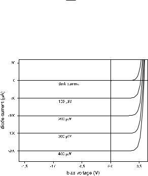
where I is the current, U is the voltage, I0 is a constant current given by the material and the temperature, e is the electron charge, m ≈ 1.5 is known as the Shockley factor, k is Boltzmann’s constant, and T is the temperature (in Kelvin). The equation di ers from that of any ordinary diode only in the additional term for the photocurrent, Ip (Fig. 8.29).
Figure 8.29: Voltage-current characteristic of a photodiode, with the absorbed light power as a parameter. For this figure, it was assumed that R = 0.5 A/W and I0 = 100 pA. At constant negative bias voltage, i.e., when one crosses the set of curves on a vertical path, the reverse current is practically identical to the photocurrent, which is proportional to the received power and almost independent of bias. For open circuit (zero current), one crosses the set of curves on a path given by the horizontal axis; then the diode generates a photovoltage which is proportional to the logarithm of the received power.
8.10. Optical Receivers |
147 |
We have to distinguish two very di erent modes of operation:
As a current source: This requires a constant bias voltage U = const. which is applied in reverse direction or may be zero. Then the photocurrent is proportional to the received light power over many orders of magnitude and almost independent of the bias voltage. The main e ect of the nonzero bias is to reduce the diode capacity and improve the temporal response.
As a voltage source: This is the operation with high impedance load so that basically I = 0. Then the diode generates a photovoltage which is proportional to the logarithm of the received light power.
While there can be uses for the voltage source mode occasionally, in our context the constant current mode is almost always preferred due to its linearity.
Unfortunately, not every photon actually generates a free charge which contributes to the photocurrent, but only a certain percentage. This percentage is called the quantum e ciency η and is an important characteristic of the detector. η is always smaller than unity because some photons fail to enter the detector (Fresnel reflection at the surface) or are not absorbed near the junction; some carriers may also recombine before they contribute to the external photocurrent.
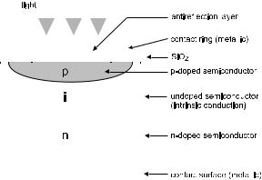
In order to obtain the most e cient absorption of the impinging light, there is usually an extra layer inserted between the p-doped and the n-doped layers, which is undoped and thus has only the intrinsic conductivity of the base material. This intermediate layer is called the i layer, as in “intrinsic conductivity”. The diode is then described as a pin diode for its three layers (Fig. 8.30). pin diodes are the most frequently used type of photodiodes and can reach quantum e ciencies up to about 90%.
To characterize photodiodes, the sensitivity (sometimes called responsivity) R is an important quantity:
|
|
|
R = |
Ip |
= |
nee |
= |
ηe |
(8.9) |
||||||
|
|
|
|
|
|
|
. |
|
|
|
|||||
Pp |
nphν |
hν |
|||||||||||||
|
|
|
|
|
|
|
|
|
|
|
|
|
|
|
|
|
|
|
|
|
|
|
|
|
|
|
|
|
|
|
|
|
|
|
|
|
|
|
|
|
|
|
|
|
|
|
|
|
|
|
|
|
|
|
|
|
|
|
|
|
|
|
|
|
|
|
|
|
|
|
|
|
|
|
|
|
|
|
|
|
|
|
|
|
|
|
|
|
|
|
|
|
|
|
|
|
|
|
|
|
|
|
|
|
|
|
|
|
|
|
|
|
|
|
|
|
|
|
|
|
|
|
|
|
|
|
|
|
|
|
|
|
|
|
|
|
|
|
|
|
|
|
|
|
|
|
|
|
|
|
|
|
|
|
|
|
|
|
|
|
|
|
|
|
|
|
|
|
|
|
|
|
|
|
|
Figure 8.30: Structure of a pin photodiode. Light enters through an antireflection layer which occupies the free aperture inside the contact ring. The remainder of the chip surface is passivated with SiO2. Absorption takes place mostly in the i layer.
148 |
Chapter 8. Components for Fiber Technology |
Here ne and np denote the number per second of electrons or photons, respectively. If η ≈ 1 one can write the numerical relation
R |
= |
e |
|
λ = |
λ(μm) |
|
A |
. |
(8.10) |
hc |
1, 24 |
|
|||||||
|
|
|
W |
|
|||||
We see that the sensitivity is of the order of 1 A/W in the near infrared.
8.10.2Materials
Silicon photodiodes are a product for mass markets. They are found in TV remote controls, in supermarket scanners, in CD and DVD players, as individual pixels in electronic cameras, etc. The band gap of silicon corresponds to λ = 1.1 μm. This means that the visible light is covered well, but for fiber optics, silicon is useful only in the first window. At the longer wavelengths of the second and third windows silicon is just simply transparent and does not absorb at all. The band edge of germanium sets on at 1.7 μm so that the entire wavelength regime of interest is covered. It turns out, though, that diodes from composite materials such as InGaAs have a similar band gap as germanium but have lower dark current and are therefore usually preferred.
8.10.3Speed
The fundamental speed limitation for a photodetector is that photo-generated carriers must transit the junction area. The maximum speed at which carriers move through the lattice depends on the material and is defined by scattering processes at the lattice atoms. Near the junction they are accelerated by the electric field of an external bias voltage. Some of the carriers, however, are not generated near the junction but in the p-layer or n-layer before or after. There the electric field strength is much lower so that these carriers must di use away; they contribute a slow portion to the electric signal. Then there is the external time constant defined by the circuitry: Unavoidable capacitances both inside and outside the diode, in combination with resistance in the circuit, defines an RC low pass. Careful construction allows to produce photodiodes with a couple of picosecond response time; commercial products are available with bandwidths up to about 60 GHz.
8.10.4Noise
Noise is a fundamental limitation to any measurement. When it comes to the detection of light with photodetectors, several noise mechanisms contribute:
Quantum noise of the light: This is a property of the light itself. Light consists of photons which arrive according to some statistics. This is reflected in the temporal distribution of photo-generated carriers and thus causes a noise contribution to the photocurrent.
dark current noise: This is a property of the detector. The e ect depends on material and temperature; it can be reduced by careful choice of material and by cooling.
8.10. Optical Receivers |
149 |
Surface leak current noise: This again is a property of the detector. Improvements can be obtained by precautions in manufacturing and possibly to some degree by cooling.
Noise from resistors and amplifiers: This is a property of the external circuitry. The e ect, also known as Johnson noise or Nyquist noise, can be minimized by optimizing the circuit.
Quantum noise turns out to be the only contribution which cannot be modified by engineering; it thus constitutes a fundamental limit. We will discuss it in more detail in Sect. 11.1.7.
8.10.5Avalanche Diodes
Avalanche diodes are the solid-state equivalent to photomultipliers. In comparison to pn or pin photodiodes, avalanche diodes are operated at a considerable reverse bias voltage. The high voltage internally generates strong electric fields which accelerate carriers to the point that upon collision with lattice atoms, they can generate more carriers by impact ionization. The photocurrent then grows like an avalanche and is amplified by a gain factor M .
It is not worth it to push M too far. The internal amplification process has its own noise component which actually grows faster than M . For each combination of avalanche diode and associated external circuit, there is an optimum gain so that the inherent noise contribution of the first amplifier stage of subsequent electronic circuitry becomes irrelevant in comparison to the signal.
Part IV
Nonlinear Phenomena in
Fibers
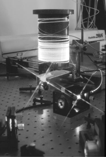
Experiment to investigate stimulated Brillouin scattering in optical fiber with visible light (ca. 590 nm). Compare Figs. 9.24, 9.25 and 9.26.

Chapter 9
Basics of Nonlinear
Processes
It is well known from acoustics that when it comes to oscillations, nonlinearity leads to the appearance of overtones. The same phenomenon also exists in optics. A first experimental demonstration succeeded in the early 1960s [45] when the generation of twice the irradiated frequency was shown in a nonlinear crystal. The mechanism relied on the anharmonicity of the oscillation of the medium’s polarization as produced by an intense light wave. Shortly thereafter, the third harmonic was also demonstrated. Since then, nonlinear optics has evolved into a field of research in its own right. Processes under study are optical rectification, parametric amplification, self-focusing, and self-phase modulation, to name just a few. Optical nonlinearity is responsible when optical properties of some material show intensity-dependent modifications, when light waves with frequencies are generated that are not present in the irradiated light, or when – speaking in more general terms – power is redistributed between di erent Fourier components of a light field. As a rule, nonlinear e ects get more pronounced as the light intensity is increased. The reverse is also true: When the light intensity is su ciently weak, nonlinear processes may safely be neglected. All of classical optics is therefore linear optics.
9.1Nonlinearity in Fibers vs. in Bulk
Nonlinear processes are also observed in optical fiber: actually, often in a more pronounced form than in bulk optics. This is due to two peculiarities of fibers: By virtue of the very small mode cross-section, there is high intensity even at moderate power. And the waveguiding allows very long interaction lengths.
These two peculiarities belong together: one could also have high intensity in bulk optics by suitably focusing down to a tiny spot. But then typically the length of the interaction zone goes down due to di raction of light. It may be best to discuss this for Gaussian beams: Beams generated by lasers typically have a Gaussian intensity profile (see Appendix D).
For a Gaussian beam, there is a characteristic length called Rayleigh range. Its significance is that near a focus the beam diameter stays nearly constant over this length. (Speaking more precisely, the beam radius widens by no more
F. Mitschke, Fiber Optics, DOI 10.1007/978-3-642-03703-0 9, |
153 |
c Springer-Verlag Berlin Heidelberg 2009

154 Chapter 9. Basics of Nonlinearity
√
than a factor of 2 over that at the beam waist.) Then the axial intensity drops by only very little (no more than a factor of 2). The Rayleigh length is given by
zR = |
πw2 |
; |
(9.1) |
|
0 |
||||
λ |
||||
|
|
|
on the other hand, the intensity at the beam waist is obtained from the total power P0 by the expression
I0 = |
2P0 |
. |
(9.2) |
|
|||
|
πw2 |
|
|
|
0 |
|
|
This is the maximum; at the end of the Rayleigh zone IR = I0/2.
Let us consider that class of nonlinear interactions which are proportional to intensity and cumulate with interaction length. Then the product of intensity and di raction-limited interaction length is a metric for the strength of the
nonlinear e ects. We obtain |
|
|
|
|
|
|
|
|
|
I0zR = |
2P |
0 |
|
πw2 |
= |
2 |
|
(9.3) |
|
|
|
0 |
|
|
P0. |
||||
πw2 |
|
λ |
|
||||||
|
|
|
λ |
|
|||||
|
|
0 |
|
|
|
|
|
|
|
This expression shows that there is no way how one could increase the strength of the nonlinear process by geometrical means, like nifty focusing arrangements or whatever.
In stark contrast, the same limitation does not occur in optical fibers. In the fiber the wave is guided, and the interaction can build up over nearly arbitrary distances. Of course, losses reduce the intensity in the fiber after some distance. We take that into account by integrating along the fiber:
L I(z)dz = |
L I0e−αz dz = |
I0 |
(1 |
− |
e−αL) = I0Le , |
(9.4) |
||
|
||||||||
0 |
0 |
|
|
α |
|
|
||
where we introduced the e ective interaction length |
|
|||||||
|
1 |
1 − e−αL . |
|
(9.5) |
||||
|
Le = |
|
|
|||||
|
α |
|
||||||
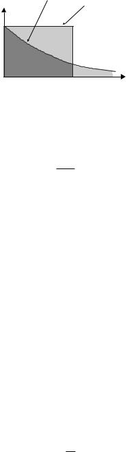
This e ective interaction length is quite important in nonlinear fiber optics. It is always shorter than the actual fiber length. This is because the power goes down so that remote parts of the fiber contribute only little to the nonlinear e ect. The definition amounts to replacing the actual decreasing power by a constant, i.e., its initial value, but limiting the interaction length to the e ective value (see Fig. 9.1). In the limiting case that the actual fiber length tends to infinity, Le tends to 1/α. In practical numbers, assuming a loss of 0.2 dB/km,
Le ,max ≈ 22 km.
In order to convert the transmitted power to intensity, we need to be more specific about the mode’s cross sectional area. We obtain it from integrating the field amplitude E(x, y) across the entire cross-section with suitable normal-
ization: |
|
|
|
|
|
|
|
dxdy 2 |
|
|
|
|
∞ |
∞ |
| |
E(x, y) 2 |
|
||||
Ae = |
|
−∞ |
−∞ |
| |
|
|
. |
(9.6) |
||
|
|
∞ |
∞ |
|E(x, y)| |
4 |
|
||||
|
|
|
dxdy |
|
||||||
|
|
−∞ |
−∞ |
|
|
|||||
Ae is the e ective mode area. If one uses the Gaussian approximation for the fiber mode, the e ective area simply becomes Ae = πw2.
9.2. Kerr Nonlinearity |
155 |
factual |
fictitious |
Intensity |
|
Leff |
Length |
Figure 9.1: Sketch to explain the concept of the e ective interaction length.
Let us wrap up: Nonlinear interaction is much stronger in fiber than in bulk. Compared with a figure of merit λ2 P0 in bulk, for fiber one finds P0Le /Ae .
The ratio of the two,
λLe ,
2Ae
is quite large. Take as typical values λ = 1 μm, Ae = 50 μm2, and Le = 20 km; then it is 2 × 10⁸. We conclude that even mild nonlinearity can have very noticeable consequences in fibers.
9.2Kerr Nonlinearity
It was shown in Chap. 3 that the refractive index can have an intensity dependence
n = n0 + n2I,
where for fused silica n2 ≈ 3 × 10⁻²⁰ m2/W. This is also known as the optical Kerr e ect. It provides a minute modification of the index by the n2 term, which does not influence the structure of the modes because n2I (nK − nM). However, the n2I term does modify the phase of the propagating light.
Consider a light wave with power P launched into the fiber. The e ective cross-sectional area of the mode is Ae . Generally, a wave of the type
cos(ωt − kz)
propagates such that after distance z = L the phase has the value kL. Therefore,
φ = kL = k0nL = k0 (n0 + n2I) L = |
2π |
n0 + |
n2 |
P L. |
|
|
|||
|
λ |
Ae |
||
This phase can be split into a linear and a nonlinear contribution:
2π
φlin = λ n0L
and
φnl = |
2π n2 |
P L = |
ω0n2 |
P L = γP L with |
γ = |
ω0n2 |
. |
||
|
|
|
|
|
|||||
λ Ae |
|
|
|||||||
|
|
cAe |
|
cAe |
|||||
We will extensively use the coe cient of nonlinearity γ below.
(9.7)
(9.8)

156 Chapter 9. Basics of Nonlinearity
With the help of a reference wave providing a phase reference, one could easily measure the nonlinear phase shift. Let, e.g., λ = 1.5 μm, n2 = 3 × 10⁻²⁰ m2/W, Ae = 40 μm2, P = 1 W, and L = 1 km. Then we obtain γ = 3.14 × 10⁻³/(Wm) and φnl = 3.14 rad which corresponds to one half of a wavelength – certainly easily measured interferometrically.
9.3Nonlinear Wave Equation
Now we will set up a wave equation which takes all relevant e ects into account. As it will turn out, it fully su ces to write an equation for the field envelope. This implies that the variable in the equation is not the field strength itself, but only its amplitude; a term oscillating at the optical frequency is removed. This is justified whenever the envelope changes much more slowly than the field, in other words, when within the duration of the shortest pulses of light there are many oscillation periods of the field. Some current research at the forefront of laser physics now pushes this limit, but there are no direct consequences for fiber-optic applications.
9.3.1Envelope Equation Without Dispersion
At first we want to see how an envelope equation is set up in a simple case. We start from the linear wave equation derived in Ch. 3 (compare Eq. 3.23)
n2 ∂2E |
= 0 |
(9.9) |
2E − c2 ∂t2 |
and use the following ansatz for E:
E(x, y, z, t) = A(x, y, z, t) ei(ω0t−β0z). |
(9.10) |
This describes a wave traveling in positive z direction, with carrier frequency ω0 and propagation constant β0 = ω0n/c. All other space and time dependence is lumped into the envelope A(x, y, z, t). We assume that these dependencies are variable only at a much slower scale, so that any spatial or temporal derivative of A, in comparison to the same derivative of the exponential term, is of order1. In physical terms this means that the envelope changes only very little during one oscillation period or over one wavelength. This approximation is justified as long as even the shortest light pulses contain several oscillations of the field.