

Fiber_Optics_Physics_Technology
.pdf11.2. Nonlinear Transmission |
229 |
Figure 11.10: Computer simulation of the equalization of power variations of solitons by filters. If a pulse has more than its normal power, it will be shorter in time and broader spectrally. In the selective filter, it experiences extra loss which will overcompensate the gain and reduce the power toward the equilibrium value. In this example, three wavelength channels are considered. Stable propagation is only obtained with the use of filters. From [82] with kind permission.
11.2.2Several Wavelength Channels
The maximum data rate of an individual wavelength channel is basically limited by the speed of electronic components as they are available. This limit is optimistically at 100 Gbit/s, and more realistically in the tens of Gbit/s. The rate may be increased somewhat by optical time division multiplexing when two or more bit streams are first converted into a sequence of pulses with fast electronics, then interleaved by using optical delays of half the clock time. There is hope that 100 Gbit/s can be obtained, but that is still a far cry from the 50 THz or so bandwidth which the fiber o ers. That tremendous spectral range can only be utilized by parallel operation of a multitude of wavelength channels, i.e., by wavelength division multiplex or WDM. The first question arising is at which spacing to place the spectral channels: should they be equidistant?
Several valid points in favor of equidistance can be brought forward:
It represents better conceptual clarity.
It is in accord with common use in radio and TV transmission.
Filters with equidistant transmission frequencies are particularly easy to construct (Fabry–Perot filters).
The counter argument is that the detrimental e ect of four wave mixing is most pronounced in this case: all newly generated frequencies sit right on top of some other channel (see Sect. 9.6). This is shown in Fig. 11.11.
Nevertheless, international standardization bodies have adopted an equidistant channel grid. The ITU3 grid uses a reference frequency of 193,100 GHz,
3International Telecommunication Union, a United Nations agency for information and communication technology issues.
230 |
Chapter 11. Applications in Telecommunications |
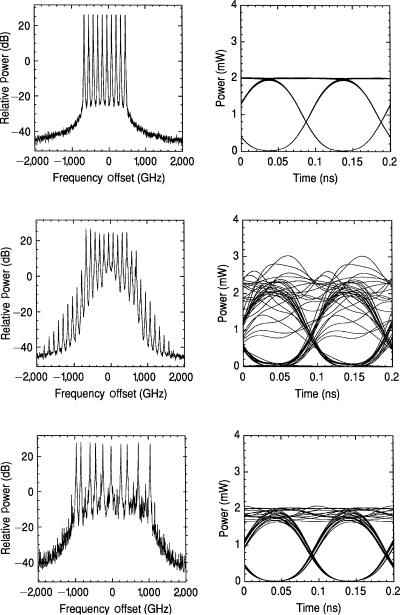
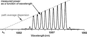
Figure 11.11: Experiment about the impact of four wave mixing in a WDM transmission system. Left : spectra, right : eye diagrams (these are explained in Sec. 11.3.2). Top row : Ten equidistant channels are launched simultaneously into a fiber. Center row : At the fiber end numerous mixing products (“combination tones”) have been generated. The eye diagram indicates severely degraded signal integrity. Bottom row : If nonequal channel separations are chosen, both the number and the strength of mixing products are reduced, and the eye diagram indicates good signal integrity (the “eye” is completely open). From [44] with kind permission.
11.2. Nonlinear Transmission |
231 |
which corresponds to a vacuum wavelength of ca. 1,552.5 nm. Starting from this frequency, there is one channel at every 100 GHz increment. Intermediate channels on a 50 GHz or even 25 GHz grid may be used. WDM using this grid is also called “dense WDM” or DWDM. This is in contrast to “coarse WDM” (CWDM) where a much wider spacing of 20 nm is used. Given the regular frequency grid, the problem arising from four wave mixing must be remedied in some other way.
Four-Wave Mixing and Phase Matching
The amount of degradation caused by four-wave mixing is also determined by the degree of phase matching of this process (Fig. 11.12). In a fiber without any dispersion, perfect phase matching of both the generating and the generated wave would be guaranteed, and mixing products and thus signal perturbation would reach a maximum. Therefore, dispersion is definitely helpful in this context. Even small amounts of dispersion reduce the e ciency of four wave mixing noticeably.
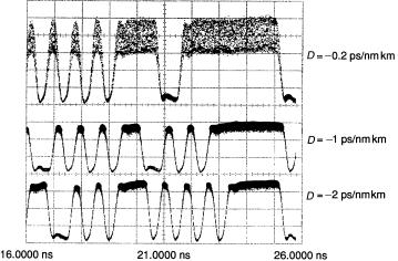
Figure 11.12: Impact of four-wave mixing on a bit sequence, compared at di erent amounts of fiber dispersion. The less dispersion, the more signal distortion. From [44] with kind permission.
11.2.3Alternating Dispersion (“Dispersion Management”)
An invention conceived for a di erent purpose is the solution to the four-wave mixing problem. Engineers had tried to solve the problem of dispersive pulse broadening by tinkering with the fiber’s dispersion. Their idea was to basically compensate the dispersion and make it zero at least as a path average by inserting segments of dispersion-compensating fiber. The latter designates dispersion-shifted fibers (see Sect. 4.5.5) which have dispersion β2 of the opposite sign as the main fiber. It turned out that a full compensation to zero is not
232 |
Chapter 11. Applications in Telecommunications |
at all desirable. In the (unavoidable) presence of fiber nonlinearity, a certain residual dispersion was found beneficial. This is, of course, rooted in soliton formation.
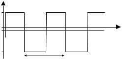
In order to reduce the detriment of four-wave mixing by the introduction of phase mismatch, it su ces to have strong local dispersion (see Sect. 9.6); even for zero-path average dispersion this end would be achieved. The idea then is to optimize dispersion along the path by judicious dispersion management (DM) to create a dispersion map. The dispersion map typically consists of a periodic alternation of fibers with di erent dispersion (Fig. 11.13); typical DM period lengths are a few tens of kilometers.
It is not at all clear that soliton-like pulses would exist in a dispersion managed fiber. After all, the periodic change of sign of dispersion is a profound perturbation which can certainly not treated as a small perturbation to the nonlinear Schr¨odinger equation. Light pulses traveling in DM fibers vary a lot in pulse duration over one DM period. Nevertheless, pulses do exist which are stabilized by the action of nonlinearity [119, 122]. This stabilization implies that after a complete DM period, the original pulse shape and width are restored. In a “stroboscopic” representation, in which the pulse shape is only shown at a particular position within the DM period, one sees a stably propagating pulse again. In a certain generalization of the concept of solitons such pulses are referred to as DM solitons. Their pulse shape is di erent from the sech shape of conventional solitons, as can be seen from Fig. 11.14. Indeed, it more closely resembles a Gaussian. On a log power scale one even discerns undulations in the wings.
The repetitive variation of dispersion brings about a further benefit: Since the pulse shape “breathes” over one dispersion period, the pulse’s phase profile breathes, too: underneath the envelope there is a chirp bending back and forth. Where neighboring pulses overlap, the phase relation varies rapidly so that interaction is mostly washed out. Moreover, for long stretches of the path, the peak power is reduced and with it the e ective nonlinearity. To make up for that, the power of the DM soliton is higher than in the comparable case of a fiber with constant dispersion equal to the path average value [142]. This so-called DM power enhancement [142, 164] provides advantages in terms of signal-to-noise ratio and also in the context of Gordon–Haus jitter [150].
Dispersion parameter β2
β+ |
βave0 |
Distance |
β– |
period |
Figure 11.13: Sketch to explain dispersion management. The fiber line consists of alternating fiber segments with positive and negative dispersion. The path average dispersion is then much lower than the local dispersion and may be close to zero.
11.2. Nonlinear Transmission |
233 |
Power
Distance
Time
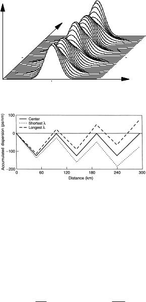
Figure 11.14: A DM soliton in a computer simulation. Two periods of the dispersion map are shown.
Figure 11.15: Accumulation of dispersion in a dispersion-managed fiber in comparison of a central channel and channels at the edges of the spectral range. From [44] with kind permission.
Due to higher-order dispersion, there is a di erent β2 value at the center frequency of each wavelength channel. Di erent channels thus experience different dispersion, both for local and path average values. This is illustrated in Fig. 11.15 where the propagation of signals in neighboring WDM channels with di erent dispersion is compared.
As a consequence, in di erent WDM channels the pulse streams have different power. If we take the unperturbed soliton of the nonlinear Schr¨odinger equation as a reference, its energy is found as
Pˆ1 = |
|β2| |
and E1 = 2Pˆ1T0 = |
2|β2| |
. |
γT02 |
|
|||
|
|
γT0 |
||
The energy is proportional to dispersion. As Fig. 11.16 shows, this relation carries over to the relation between energy and path average dispersion of DM solitons [113]. Meanwhile fibers with an inverse trend of dispersion (inverse β3) have been suggested in order to obtain a flat resulting dispersion so that power di erences are equalized.
In a similar fashion, gain must be equalized, too. The spectral gain curve of Er-doped fibers as shown in Fig. 8.19 is not at all flat. By tweaking fiber design, an essentially flat range of more than 80 nm has been demonstrated. A
234 |
Chapter 11. Applications in Telecommunications |
Figure 11.16: Nine WDM channels of a DM system are operated with signals of the same bit rate. After a su ciently long distance, the power in each channel adjusts itself according to the path average dispersion of that channel. This is the same scaling behavior as known from “ordinary” solitons. From [113] with kind permission.
more broadband alternative is to use gain by means of the Raman e ect; see e.g., [124].
At the turn of the millennium, researchers had succeeded to transmit several terabits per second over a single fiber. Engineers describe these systems as chirped RZ, i.e., they realize that the pulses have the chirp that a soliton acquires in a dispersion-managed fiber, yet they typically avoid to speak of solitons. This seems to be a case of two cultures which, meaning the same thing, call it a by di erent name.
For many years, the telecommunications industry has been driven by everincreasing demands for transmission capacity. It is a fact of life that fiber is a nonlinear transmission medium; therefore one only has the choice of either avoiding the impact of nonlinearity by using wide area fibers and low signal power, or to embrace it and accept nonlinear chirp–whether one calls that format “chirped RZ” or “soliton” is of lesser importance. This author believes that solitons are the future of optical telecommunications. If this turns out to be true, maybe one day kids will hear about solitons in school!
11.3Technical Issues
11.3.1Monitoring of Operations
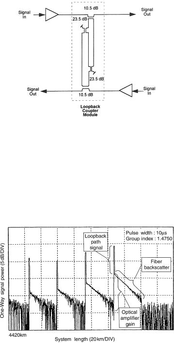
In commercial service, a permanent monitoring of system integrity is mandatory. This is done in the following way: The intermediate amplifiers along the line are combined with so-called loopback modules. These consist of four fiber couplers as shown in Fig. 11.17. In this arrangement the signal stream can pass, but a minor portion of it is branched o , attenuated by 45 dB, and sent back toward where it came from. This weak signal does not interfere with other data streams.
Somewhere among the multitude of WDM channels a pseudo-random sequence is transmitted. By way of correlation measurement, the return signal can be detected in spite of being weak. Such monitoring allows to detect additional losses due to damage or whatever cause. The damage can also be localized because the return signals from di erent loopback modules arrive with di erent delay.
11.3. Technical Issues |
235 |
Figure 11.17: A loopback module serves to monitor a dual-fiber line during operation with life tra c. After [169] with kind permission.
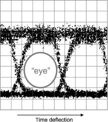
In addition, loopback modules are built such that backpropagating light from Rayleigh scattering can bypass the amplifiers so that OTDR measurements may be performed. For extremely long distances, one combines OTDR with coherent detection to increase sensitivity. With these measures the entire fiber length can be monitored, in part during life data tra c on a reserved channel, and with improved sensitivity during a routine maintenance interval. Figure 11.18 shows an example of monitoring a fiber of about 4,400 km length [83].
Figure 11.18: OTDR measurement of a very long fiber line including several amplifiers. From [43] with kind permission.
236 |
Chapter 11. Applications in Telecommunications |
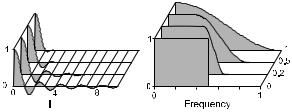
Figure 11.19: An eye diagram is obtained by displaying the bit stream over time with synchronization to the clock rate. The upper and lower levels of the binary signal and the steep slopes at the beginning and end of the bit slot can be assessed quickly and conveniently; if the eye is wide open, one may expect error-free reception.
11.3.2Eye Diagrams
One of the simplest and most e cient ways to test the quality of transmission is to inspect the so-called eye diagram. The name refers to an oscilloscope display of the bit stream such that the horizontal deflection is synchronized with the clock rate. In principle, all slopes (rising as well as falling) are then at the same position on the screen; in between, in principle there is either the upper or the lower level. Therefore, in the middle of the picture, there should be an empty area, which is referred to as the “eye.” All kinds of signal impairments conspire to close the eye (Fig. 11.19): The slopes of the pulses may be smeared out, e.g., when the light source or detector have insu cient bandwidth, fiber dispersion is unchecked, or by timing jitter. Then the eye is narrowed horizontally. The upper and lower level may not be maintained, or there may be excessive noise or channel crosstalk: Then the eye is narrowed vertically. A wide open eye is an instant indication of good signal integrity.
11.3.3Filtering to Reduce Crosstalk
Intersymbol interference can lead to channel crosstalk and can be a severe perturbation, but by judicious choice of the frequency response of the transmission
11.3. Technical Issues |
237 |
chain it can be nearly eliminated. The reader is reminded that most filters, in particular those with steep slopes of their spectral transmission, have a nonmonotonous step response. The trick then is to select a frequency response such that in the distorted filtered temporal shape there are zeroes at multiples of the clock period. If this is the case, then the crosstalk is eliminated. For example, a filter with step response
u(t) = |
sin(πt/T ) |
= sinc |
|
t |
|
(11.11) |
|
πt/T |
|
|
|||||
|
|
T |
|
||||
has the desired property. With this step response, it has a frequency response
T : f < 1/2T,
U (f ) =
0: f > 1/2T.
+∞
(T appears here from a normalization −∞ U (f ) = 1.) Such filter with “vertical” slope, usually referred to as a brick wall filter, cannot be built because it would require an infinite number of selective elements. Also, a filter with time-symmetric response defies causality (any e ect takes place only after the cause) and thus cannot be built with ordinary hardware.
This is too bad because such a filter would make it possible to optimize bandwidth use according to the sampling theorem and also because it would reject all out-of-band noise. So can one still make use of these ideas?
One can approximate the step response of the acausal filter quite well if one does not perform the filtering in real time but accepts a certain latency. It turns out, fortunately, that a latency of only a few clock periods su ces. The infinite “brick wall” slope becomes unnecessary when using a raised cosine filter, which is its generalization with rounded slope (Fig. 11.20).
T
Figure 11.20: Explanation of the raised cosine filter. Parameter β (increasing from front to back) sets the sharpness of transition from pass band to rejection band. The zeroes in the temporal response remain centered on the positions of the adjacent bits so that channel crosstalk is eliminated.

238 |
|
|
|
|
|
Chapter 11. |
|
|
Applications in Telecommunications |
||||||||||||||||||
If the filter has the frequency response |
|
|
|
|
|
|
|
|
|
|
|
|
|
||||||||||||||
|
|
|
|
|
|
|
|
|
|
|
|
|
|
|
|
|
|
|
|
|
|
|
1 |
− |
β |
||
|
|
T |
|
|
|
|
|
|
|
: |
|
|
|
0 |
≤| |
f |
|
|
|
, |
|||||||
|
|
|
|
|
|
|
|
|
|
|
|
|
2T |
|
|||||||||||||
|
|
|
|
|
|
|
|
|
|
|
|
|
|
|
|
|
|
|
|
|≤ |
|
|
|
|
|||
|
|
|
|
|
|
|
|
|
|
|
|
|
|
|
|
|
|
|
|
|
|
|
|
|
|
|
|
U (f ) = |
|
|
|
|
|
|
|
|
|
|
|
|
|
|
|
|
|
|
|
|
|
|
|
|
|
(11.12) |
|
|
|
|
|
|
|
|
|
|
|
|
|
|
|
|
|
|
|
|
|
|
|
|
|
|
|||
|
|
|
|
|
|
|
|
|
|
|
|
|
|
|
|
|
|
|
|
|
|
|
|
|
|
|
|
|
|
|
T |
πT |
|
|
1 |
− |
β |
1 |
− |
β |
|
|
f |
1 + β |
|||||||||||
|
|
|
|
1 + cos |
|
|
f π |
: |
|
|
|
|
|
|
|
|
|
, |
|||||||||
|
|
2 |
|
|
β − |
|
|
2β |
|
|
|
|
|
2T ≤| |≤ 2T |
|
|
|||||||||||
|
|
|
|
|
|
|
|
|
|
|
|
|
|||||||||||||||
|
|
|
|
|
|
|
|
|
|
|
|
|
|
|
|
|
|
|
|
|
|
|
|
|
|
|
|
|
|
|
|
|
|
|
|
|
|
|
|
|
|
|
|
|
|
|
|
|
|
|
|
|
|
|
|
it follows that it has the step response |
|
|
|
|
|
|
|
|
|
|
|
|
|
|
|
|
|
||||||||||
|
|
|
|
u(t) = |
|
sin(πt/T ) |
|
cos(βπt/T ) |
, |
|
|
|
|
(11.13) |
|||||||||||||
|
|
|
|
|
πt/T |
|
|
|
|
|
|
||||||||||||||||
|
|
|
|
|
|
|
|
|
|
1 − (2βt/T ) |
|
|
|
|
|
|
|||||||||||
which in turn is a generalization of a sinc function. By tweaking the parameter β, one can fine-tune the sharpness of the transition from pass band to rejection band. Such filters can be made to a good approximation and allow to have a well-defined pass band to keep noise in check. At the same time, they cancel channel crosstalk from intersymbol interference.
11.4Telecommunication: A Growth Industry
Nothing displays the increasing globalization as clearly as the increasing demand for long-distance communications lines. For many years, there has been an annual growth by some 20–30%. The race to keep up with the rising demand is fueled by the incentive of money to be made; some of that money is well invested in research to advance the technology involved. We now give a historical sketch of the development of telecommunications.
11.4.1Historical Development
1851: The first undersea cable commences service. It crosses the English Channel, connecting Dover and Cape Gris Nez, and it will work well for 24 years.
1858: The first transatlantic cable begins operation, but it is broken after only 1 month.
1927: The first transatlantic telephone connection is inaugurated. It is based on radio transmission in SSB mode between New York and London.
1956: The first transatlantic telephone cable (“TAT-1”) takes up service. Its coaxial cable can accommodate 48 simultaneous telephone channels in analog format. The amplifiers use electron tubes (transistors are invented only shortly before and are not mature yet). In a sophisticated scheme, even the silent intervals in natural conversation are used for transmission of other channels, a scheme called TASI for “time-assignment speech interpolation.” This technology is very successful so that a few years later more cables follow, which use the same basic technology but an increasing number of channels. The seventh of these (TAT-7, with 4,000 telephone channels) is the last of its kind. It is commissioned in 1983 and can handle 4,200 simultaneous telephone channels. TAT-1 is decommissioned in 1978, TAT-7 in 1994.