

Fiber_Optics_Physics_Technology
.pdf4.2. Waveguide and Profile Dispersion |
53 |
4.2Waveguide and Profile Dispersion
In addition to material dispersion Dm, in fibers there is waveguide dispersion Dw. Without explicitly deriving the result, we state that for step index fibers, it can be calculated from [50, 120]
|
V nK |
|
d2 |
|
|||
Dw = − |
|
|
|
|
|
(V b) , |
(4.29) |
|
λc |
dV 2 |
|||||
where |
β2 − kM2 |
|
|
|
|||
b = |
. |
|
|||||
|
|
kK2 − kM2 |
|
||||
For very large V number, the dimensionless quantity b tends to b = 1; at the cuto of each mode there is b = 0.
The reason for the waveguide contribution can be intuitively understood by noting that for increasing wavelengths, the field extends more and more into the cladding so that the light wave experiences more and more of the cladding index, rather than just the core index (Fig. 4.3).
c 
c


Figure 4.3: The travel time of a signal in a fiber is obtained from taking a suitably weighted average of travel time pertaining to core and cladding material. At short wavelength, light is guided predominantly in the core; at long wavelength, overwhelmingly in the cladding. The zero-dispersion wavelength (corresponding to minimum travel time) therefore shifts toward longer wavelength, compared to the core material alone.
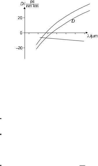
If one takes into account that on top of this is also not constant but depends slightly on wavelength, one obtains what is called profile dispersion or di erential material dispersion Dp. This contribution is usually small and will not be further discussed here. Below we will refer to the sum D = Dm +Dw +Dp (Fig. 4.4).
Specifications by fiber manufacturers quote either D (and sometimes S) or β2 (and sometimes β3) at specific wavelengths. The values given refer to the total; relative contributions of material, waveguide, and profile dispersion are not normally provided. Conversions (4.18), (4.27) and (4.28) remain valid when indices “m” are dropped.
54 |
Chapter 4. Chromatic Dispersion |
Dm
1.0 |
1.5 |
Dw
Figure 4.4: Total dispersion D results from the material contribution of the core Dm and the waveguide contribution Dw. The zero-dispersion wavelength is shifted by Dw with respect to what would be expected from Dm alone.
4.3Normal, Anomalous, and Zero Dispersion
Let us consider some typical numerical values. Figure 4.2 shows the refractive index for fused silica as obtained from a Sellmeier’s equation. We make the following observations:
Throughout the visible and near infrared, dn/dλ < 0. This implies that ngr = n − λ(dn/dλ) > n. The group index is larger than the phase index. In the near infrared, ngr is nearly constant at about ngr = 1.46 .
The refractive index n(λ) has an inflexion point at λ ≈ 1.27 μm. At this point, group delay is minimal and Dm = β2 = 0, so that this point is referred to as zero-dispersion wavelength. Strictly speaking, this commonly used term is slightly incorrect since it is only the leading order in the series expansion of the dispersion that vanishes here. All higher-order terms still contribute. Below we will call this particular wavelength λ0.
d2n
For λ < λ0 and in the visible in particular, dλ2
D = −(λ/c)(d2n/dλ2) is negative, while for λ > λ0, D is positive. Historically, the visible range was investigated first and therefore the trend observed there was considered “normal.” Then, the case D < 0 is called “normal dispersion.” Correspondingly, the opposite case D > 0 is called “anomalous dispersion.” If the fiber is used in the second window near 1.3 μm, there is a minimum of the dispersion (D ≈ 0), while in the third window around 1.5 μm there is anomalous dispersion.
Let us emphasize again: We are here concerned with one type of dispersion exclusively and that is the group velocity dispersion. For the dispersion of the refractive index similar terminology is used: There, too, one has “normal” and “anomalous” dispersion. “Normal” refers to the case that the index decreases

4.4. Impact of Dispersion |
55 |
toward longer wavelengths, the standard situation in the transparent range of most materials. The opposite only occurs near atomic resonance frequencies; that is then called anomalous dispersion (of the index). Unfortunately, some authors do not always make it entirely clear just which type of dispersion they refer to, so that occasionally confusion may arise.
The waveguide contribution to the total dispersion is negative throughout the visible and near infrared. A typical value for standard fibers is −2 ps/(nm km). At long wavelengths, it acts opposite to the material dispersion. Consequently, the zero-dispersion wavelength in standard fibers is slightly shifted with respect to bulk fused silica, toward longer wavelengths by typically about 20–30 nm. According to a CCITT1 standard in e ect since 1984, the dispersion of fibers for telecommunication purposes shall be bounded as follows:
|D| ≤ 3.5 ps/nm km |
for 1, 285 nm ≤ λ ≤ 1, 330 nm, |
|
|
|D| ≤ 20 ps/nm km |
at λ = 1550 nm. |
|
|
Near 1.55 μm, a |
value of D |
= 18 ps/nm km is |
typical. (According to |
Eq. (4.27) this corresponds to β2 |
= −23 ps2/km.) |
This value will generate |
|
a propagation time di erence between two wavelength components that are 1 nm apart, which after a distance of L = 10 km reaches δτ = 180 ps. The zero-dispersion wavelength near 1300 nm provides minimal spread in propagation time in the second window. Third-order dispersion varies not as much with wavelength as the second-order term. Typical numbers are S(λ0) = 0.085 ps/nm2 km, corresponding to β3(λ0) = −0.08 ps3/km.
As we will see shortly, the shift of the zero-dispersion wavelength by the waveguide dispersion can be intentionally increased. This allows to make fibers with custom-designed zero-dispersion wavelength in the infrared at wavelengths beyond the zero of pure fused silica.
4.4Impact of Dispersion
Consider the propagation of a light pulse which we think of as being generated by taking a monochromatic oscillation
ˆ −
E cos(ωt βz)
and multiply (modulate) it with an envelope function. For the latter a reasonable choice is a Gaussian:
e− |
t2 |
|
2 |
(4.30) |
|
2T0 . |
The temporal profile of the intensity (irradiance) or power of a pulse so generated is
I(t) = I0 e−(t/T0)2 . |
(4.31) |
1Comit´e Consultatif International T´el´egraphique et T´el´ephonique. This committee is now called ITU-T, a subunit of the International Telecommunication Union, which is a United Nations agency for information and communication technology issues.

56 |
Chapter 4. Chromatic Dispersion |
Here I0 is the peak value of the intensity and T0 the pulse duration. Note that there is not a unique way to specify pulse duration: T0 refers to the time interval between the peak and the point where the intensity has dropped to 1/e of the maximum. However, experimentalists and technicians often prefer the use of the half width of the pulse, i.e., the time elapsed between the points, where the power or intensity takes 1/2 of the peak value. This half width is often
denoted by “FWHM” (full width at half maximum); we will designate it by τ .
√
The conversion for a Gaussian is τ = 2 ln 2 T0.
After propagation over fiber length L, both pulse duration and peak power are modified. One can show that the pulse duration now is
|
|
|
|
|
L |
|
2 |
|
|
|
TL = T0 1 + |
|
|
, |
(4.32) |
||||||
LD |
||||||||||
|
|
|
|
|
|
|
|
|||
where |
T 2 |
|
|
|
|
|||||
LD = |
|
|
|
(4.33) |
||||||
|
0 |
|
|
|
|
|
||||
|β2| |
|
|
|
|||||||
is a characteristic length called the dispersion length. After distance LD, the |
|||||
pulse duration has increased by |
√ |
|
|
After considerably longer distance, the |
|
2. |
|||||
pulse duration grows in proportion to distance as |
|
||||
L LD |
|
TL = |β2|L/T0 . |
(4.34) |
||
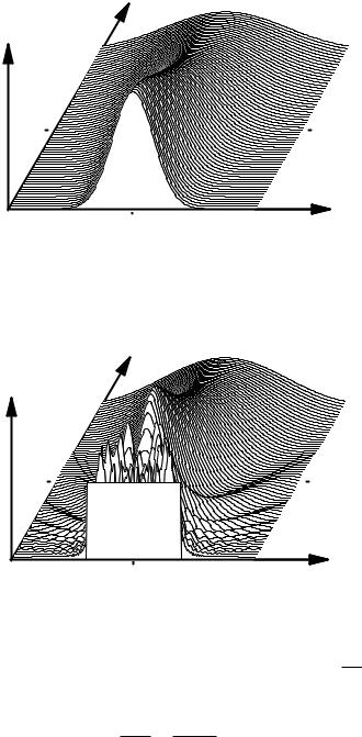
The shorter initially, the longer in the end! We point out that there is a very close analogy with di raction, the transverse spreading of a narrow fan of light rays, and dispersion, the longitudinal spreading of a short light pulse. Far-field di raction (Fraunhofer di raction) is the most transparent case: The spread increases in proportion to distance, i.e., at a constant angle of divergence. The functional form of the fan of rays is given by the Fourier transform of the initial shape and remains unaltered; only scale factors evolve. In the near field (Fresnel di raction) the situation is more involved, but for a Gaussian it is true that its shape is maintained except for scale factors (Fig. 4.5). Gaussians display a particularly simple behavior under this transformation, which is of course why we considered this special shape.
This close analogy becomes especially clear when we replace the Gaussian envelope of Eq. (4.30) with a rectangular envelope
|
|
0: |
t < |
|
− |
T0 |
, |
|
|
|
||
|
|
2 |
|
|
||||||||
|
|
|
|
T |
|
|
T |
|
|
|||
|
|
|
|
0 |
|
|
|
0 |
|
|||
|
|
|
|
|
|
|
|
|
|
|||
I(t) = |
|
|
|
|
|
|
|
|
|
|
|
|
|
1: |
− 2 |
|
≤ t ≤ + 2 , |
||||||||
|
|
0: |
t > |
|
|
T0 . |
|
|
|
|
||
|
|
|
|
|
|
|
|
|
|
|
|
|
|
|
|
|
|
|
|
2 |
|
|
|
|
|
|
|
|
|
|
|
|
|
|
|
|
|
|
|
|
|
|
|
|
|
|
|
|
|
|
|
This is certainly not a realistic proposition, but it comes closest to resemble di raction at a slit. Initially certain undulations are generated near the steep slopes; as propagation proceeds, they spread out. After some wiggling and interfering, the pulse shape eventually approaches the functional form of (sin(x)/x)2 (see Fig. 4.6). The close relation to di raction at a slit, and the transition from near field to far field, is quite obvious here.
In Eq. (4.33) we used β2 and T0. However, experimentalists and technicians often prefer to use the dispersion parameter D and the full width at
4.4. Impact of Dispersion |
57 |
position |
power |
time |
Figure 4.5: Dispersive broadening of a Gaussian pulse. The figure shows a pulse with initial width (FWHM) of 0.5 ps as it propagates over a distance of 21 m and widens in the process. Its peak height is reduced because energy is conserved. Fiber dispersion was chosen here as β2 = −18 ps2/km and β3 = 0.
position |
power |
time |
Figure 4.6: Dispersive broadening of a rectangular pulse. This case is purely academic, but it shows in particular clarity how steep slopes of the initial shape are deformed strongly by dispersion.
√
half maximum τ . Using the conversions τ0 = τ (L = 0) = 2 ln 2 T0 and |β2| = |D|λ2/(2πc) as given above, we can write the relevant term in Eq. (4.32) as follows:
L |
= |
L|β2| |
= |
L|D|λ2 |
|
2 ln 2 |
. |
(4.35) |
|
T02 |
τ02 |
|
|||||
LD |
|
|
|
πc |
|
|||
The first fraction on the RHS specifies the fiber(L, D) and the light signal (λ, τ0). The second fraction contains only constants and is thus independent of the specific situation. Its value equals 1.4709 × 10⁻⁹ s/m. If one now inserts L in

58 |
Chapter 4. Chromatic Dispersion |
km, D in ps/nm km, λ in μm, and τ0 in ps, units combine to give an additional numerical factor of 109, and we can write
|
|
|
|
|
|
|
|
τL = τ0 |
1 + |
|
1.47L|D|λ2 |
2 . |
(4.36) |
||
|
|
|
|
τ 2 |
|
||
|
|
|
0 |
|
|
|
|
This equation contains directly measurable quantities in technically common units and is thus of practical value. The “magic number” 1.47 is valid for Gaussian pulses; for other shapes somewhat di erent values apply. For example, the hyperbolic secant squared shape (sech2) often encountered for solitons requires a value of 1.87.
Dispersive broadening limits the information-carrying capacity because pulses must be kept at su cient temporal distance from each other. The highest capacity would be obtained at the lowest dispersion, which in turn is found at the zero-dispersion wavelength. This is why a large fraction of all installed fibers is designed for operation in the second window near 1.3 μm. However, this apparently obvious conclusion was arrived at in the framework of the linear approximation, i.e., at su ciently small powers or intensities. Nonlinear e ects (Chap. 9 .) will modify the result and maximize capacity at a di erent condition.
4.5Optimized Dispersion: Alternative Refractive Index Profiles
So far we have dealt with fibers with a step index profile. One might note that there never is such a thing as an exact step index fiber. Due to manufacturing limitations, there are slight deviations from the ideal profile, e.g., quite often there is a central dip of the index caused by a certain process step (see Sect. 6.2).
More importantly, fibers are often used with a refractive index profile that is more complex. When such fibers are produced, the objectives are to (a) maintain the single-mode property, (b) maintain low loss, and (c) add more design degrees of freedom for controlling and tailoring the dispersion.
4.5.1Gradient Index Fibers
In the context of multimode fibers, we have already mentioned a radial dependence of the index according to
|
1 − 2Δ |
r |
|
α |
|
|
n(r) = nK |
|
; |
(4.37) |
|||
a |
||||||
single-mode fibers can be endowed with a similar gradient index profile. Ray optics fails to provide a good interpretation in this case. A wave-optic calculation yields the following:
α= ∞: This limiting case is the step index profile (SI profile). The cuto of the second (LP11) mode is at V = 2.405.
α= 2: For a parabolic profile (Fig. 4.7) the cuto of the second mode shifts to V = 3.518.
4.5. Optimized Dispersion |
59 |
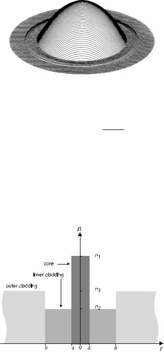
Figure 4.7: Pseudo-3D rendering of the refractive index profile. Across the circular section the index is plotted in vertical direction. From [102].
α = 1: This is a triangular profile, hence the name “T fiber” (as in triangular). Here the cuto of the second mode is even higher. As a rough approxi-
mation, the cuto occurs at V ≈ 2.405 1 + 2/α.
4.5.2W Fibers
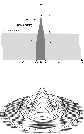
There may be an additional zone between core and cladding having its own lower refractive index (Fig. 4.8). Then a cross-sectional index profile roughly resembles the letter W; hence the name “W fiber” (Fig. 4.9). An alternative name is “DIC fiber” for depressed-index cladding fiber. This profile provides ample freedom for designing the dispersion variation.
Figure 4.8: Schematic shape of the index profile of a W fiber (depressed-index cladding profile). There are three indices for core, inner, and outer cladding, labeled here as n1, n2, and n3, respectively.
60 |
Chapter 4. Chromatic Dispersion |
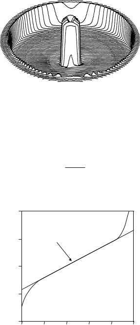
Figure 4.9: Pseudo-3D rendering of the refractive index profile of a W fiber (depressed-index cladding profile). From [102].
For this profile, we define a V number
|
2π |
|
|
|
||
V = |
|
a n12 − n32 |
||||
λ |
||||||
and an index contrast |
|
n2 |
− n3 |
|
||
R = |
. |
|||||
n1 |
||||||
|
|
− n3 |
||||
(4.38)
(4.39)
It is a remarkable property of this profile that – in marked contrast to the step index profile which guides the fundamental mode down to arbitrarily small V
V
2.5
2.0V = 1.075 (1 – R)
1.5
1.0
0.5
0 |
– 0.2 |
– 0.4 |
– 0.6 |
– 0.8 |
– 1.0 |
R
Figure 4.10: For fibers with W profile, V can be controlled by the index contrast. Over a certain range a linear approximation is appropriate. From [116] with kind permission by IEEE.
4.5. Optimized Dispersion |
61 |
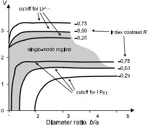
Figure 4.11: For fibers with W profile, the cuto behavior can be controlled through the ratio of radii b/a. There is even a cuto for the fundamental mode LP01 as soon as b/a is su ciently larger than unity. For example, at R = −0.5 and at b/a = 3, the fiber is single mode only in the interval 1.8 ≤ V ≤ 3.0. For V ≥ 3.0 there is the additional LP11 mode, and for V ≤ 1.8 there is no guided mode at all. After [116] with kind permission by IEEE.
at least in principle – here the fundamental mode has a finite lower cuto . Approximately and for medium values of the index contrast (Figs. 4.10 and 4.11), at the fundamental mode cuto one has
V0 ≈ 1.075 (1 − R) . |
(4.40) |
Note that in the limit n2 → n3 which reproduces the step index profile, this simple linear trend is not maintained, and V goes to zero in accord with our earlier result for step index fibers.
4.5.3T Fibers
T fibers or triangular fibers are popular because the dispersion trend is more favorable than in step index fibers, while losses are, if anything, even lower. The latter can be traced back to the interface between core and cladding: for the sudden transition of glass composition there is an enhanced chance of mechanical stress which is mitigated by a more gradual transition. Figures 4.12 and 4.13 show a modified T profile which is really a combination of T and W profiles.
4.5.4Quadruple-Clad Fibers
It is possible to add more concentric cladding layers, and increasingly the number of design degrees of freedom rises in the process. Quite frequently a quadruple-clad fiber is used (see Figs. 4.14 and 4.15). The core is typically doped with germanium and thus has a raised refractive index. The first cladding zone
62 |
|
|
|
|
|
|
|
|
Chapter 4. Chromatic Dispersion |
||
|
|
|
|
|
|
|
|
|
|
|
|
|
|
|
|
|
|
|
|
|
|
|
|
|
|
|
|
|
|
|
|
|
|
|
|
|
|
|
|
|
|
|
|
|
|
|
|
|
|
|
|
|
|
|
|
|
|
|
|
|
|
|
|
|
|
|
|
|
|
|
|
|
|
|
|
|
|
|
|
|
|
|
|
|
|
|
|
|
|
|
|
|
|
|
|
|
|
|
|
|
|
|
|
|
|
|
|
|
|
|
|
|
|
|
|
|
|
|
|
|
|
|
|
|
|
|
|
|
|
|
|
|
|
|
|
|
|
|
|
|
|
|
|
|
|
|
|
|
|
|
|
|
|
|
|
Figure 4.12: Schematic refractive index profile of a fiber with triangular core profile, shown with a depressed inner cladding. Again, three indices n1, n2, and n3 need to be distinguished.
Figure 4.13: Pseudo-3D rendering of a triangular profile, here with more complex cladding composition. From [102].
can be doped with phosphorus and fluorine and has lowered index. In the second and third cladding zones germanium and phosphorus/fluorine are repeated with suitable concentrations. The outermost cladding can then remain undoped fused silica.
4.5.5Dispersion-Shifted or Dispersion-Flattened?
There is an important distinction between dispersion-shifted and dispersionflattened fibers. In comparison to a step index fiber, by using a triangular core profile with a depressed cladding zone as in Fig. 4.12, one can achieve a shift of the dispersion curve toward longer wavelengths (Fig. 4.16). The zerodispersion wavelength can thus be moved all the way to 1550 nm if desired. Using a quadruple-clad design one can even achieve a very low dispersion simultaneously at both 1300 and 1550 nm by bending the dispersion curve flat.