Fiber_Optics_Physics_Technology

Part I

Introduction

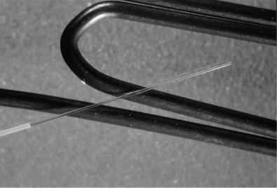
An optical fiber in comparison to a paper clip. On the far left, part of the fiber’s plastic coating is visible; mostly the fiber is bare, though. Only a small fraction of its diameter of 125 μm near the fiber axis serves the waveguiding directly.

Chapter 1

A Quick Survey

Visual, and hence optical, communication is older than language. Hand signals, waving of the arms, and fire and smoke signals are basic means of communication, and except under detrimental environmental conditions like pitch-black darkness or fog, they are useful over longer distances than shouting; besides, they are not thwarted by noises like surf at the seashore.

Normally we communicate verbally. Hence, when optical means are employed, there is a necessity to agree on a code that serves to translate the visible signs into a meaningful message.

Certain signs of nontrivial meaning are understood universally and even independent of language: consider the handwaving sign for “come here.” On the other hand, the vocabulary of such signs is too limited to convey truly complex messages. Codes that represent smaller units of language – syllables, phonemes, or individual letters – are much more universal. The best-known example may be the Morse alphabet. Of course, it is mandatory that both sender and receiver of the transmitted message have agreed on the code ahead of time. In today’s computerized environment, codes of various kinds are of tremendous importance.

The range (maximum distance) of optical transmission of messages can be increased by concatenation of several shorter spans. In the Greek tragedy of Agamemnon (part of The Oresteia), Aeschylus (ca. 525–456 BCE) mentions how the news about the fall of the city of Troy was transmitted over 500 km to Agamemnon’s wife, Clytemnestra [16]. Also, fire and smoke signals were transmitted from post to post along the Great Wall of China as early as several centuries BCE; during the Ming dynasty 1368–1644, this link stretched for over 6000 km from the Jiayuguan Pass outpost to the capital, Beijing (and on to the east). In modern times, the first systematic attempts at optical telecommunication took place in France, where Claude Chappe constructed the first optical telegraph in 1791 [73]. It is little known that Chappe initially worked with electrical devices, but decided that optical ones were advantageous. The French National Convention was initially decidedly disinterested, but in 1794 the first state-operated telegraph line was started between Lille and Paris. Every few kilometers, there were repeater stations called semaphors using mechanically movable pointers or hands; they were observed from neighboring stations, aided by telescopes. This system allowed to send messages from Paris to Lille in just 6 min – corresponding to twice the speed of sound. Later, a whole grid of such

c Springer-Verlag Berlin Heidelberg 2009

lines was built across all of France, eventually reaching a total length of 4800 km (Fig. 1.1). As is often the case with new technology, the first application was a military use. Napoleon I successfully used it for his trademark rapid military campaigns and had a portable system built for his campaign against Russia. Sweden also built a comparable network, and the UK and other countries followed suit. Around 1840, this technology saw its climax and was very common. Also the USA had a few lines (“Telegraph Hill” remains a San Francisco landmark to this day).

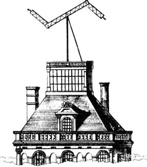
Figure 1.1: A semaphor atop the roof of the Louvre. From [10].

However, the age of electric telegraphy dawned by then. Half a century after their introduction, optical telegraphs were phased out. As it turned out, electric systems were less prone to service interruption in case of inclement weather. Beginning ca. 1858, progress in the electric technology finally added superior speed as a further advantage of electric systems.

One should note that the heyday of the electric telegraph coincides with the age of colonialism. That is relevant insofar as it speaks to the interplay between technical and political developments. Colonial powers supported the new technology because it gave them much better control over their dependencies. One hardly overestimates the importance of fast message transmission for the political situation of the day. We are denizens of the twenty-first century and find it impossible to imagine the absence of electronic means of data transmission.

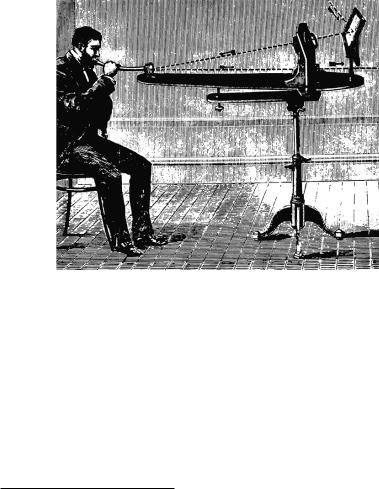
For a long time, in the development of the technology, optical systems took a back seat. It is therefore amusing to note that the inventor of the telephone, Alexander Graham Bell,1 was strongly interested in optical means of transmission. In 1880, he introduced what he called the photophone, a contraption in which the sound pressure waves emanating from a speaker’s lips moved a mirrored membrane in such a way that a light beam directed onto it got intensitymodulated (Fig. 1.2). On the receiver side, a selenium photocell served as a converter of the received light wave back to an electric current that could be converted to audible sound with an ordinary headphone. Both transmitter and receiver were thus realized with optical means; only at the receiver, electrical gear was also involved.

Figure 1.2: Alexander Graham Bell’s photophone: Sunlight is directed onto a membrane that vibrates as it is agitated by the sound from the speaker. The modulated light beam is transmitted and eventually demodulated with a Selenium photo cell. Reproduced with permission from Alcatel-Lucent.

This system had the unsurmountable disadvantages that a good light source was not available – after all, the sun does not always shine – and that the transmission span was vulnerable to adverse atmospheric conditions: rain, snow, and fog. Bell had no way of knowing, of course, that 100 years later both problems would be solved through the introduction of practical lasers and optical fibers. Only after both these novelties were available, optical data transmission had a new chance. Indeed, the chance turned into a success story probably second to none.

1Bell was not the only, indeed not even the first, inventor of the telephone. He filed his patent in 1876, but the Italian technician Antonio Meucci (who lived in New York) had demonstrated a working model as early as 1860 and the German teacher Philip Reis built another version in 1861. The American Elisha Gray had the bad luck of filing his patent all of 2 h after Bell. However, Bell is usually cited as the inventor because he won all legal patent battles, developed the scheme into a marketable product, and had the wherewithal to introduce it to the public.

In the 1960s, the laser had just been invented, and the prospect of having workable, practical devices in the near future became realistic. At that time, the propagation of laser beams through the open atmosphere in the presence of various atmospheric conditions was studied systematically and at di erent wavelengths [35]. As an alternative, there were also attempts to guide light in ducts. This made it necessary to refocus the beam frequently. In one approach, this was attempted with a large number of lenses that were inserted into the beam path in certain short distances. In a di erent try, researchers experimented with a distributed lens: This involved a gas-filled duct in which a radial temperature gradient was generated and maintained. The temperature gradient, by way of expansion of the warmer gas at the center, gave rise to a refractive index profile that acted as an e ective lens. The same basic idea but in a “solid-state” version is used today in the so-called gradient index fibers (see below). It is illuminating to assess the state of the art at that time as described in an account given by Kompfner [90].

There were obvious disadvantages in these approaches: It is not easy to form bends in such light guides – the bend radius had to be hundreds of meters! Also, installation and operation were quite costly. Only a few years later there were optical fibers: thin strands of glass, flexible enough to be coiled around a finger, and as inexpensive as copper wire, with no maintenance cost because the light-guiding index profile is built right into the fiber structure!

At that time, it was well known that microwaves can be sent through waveguides that are easy to produce. It was also known that glass can be spun into thin threads, that such threads are flexible, and even that they can guide light. However, transmission of information through such fibers was impossible due to the high transmission loss, a property shared by all transparent solid materials known at that time. Di erent materials had been studied, but among the best suited was glass with a chemical composition given by SiO2, known as fused silica. But even in fused silica, light was attenuated by at least one third after a distance no longer than 1 m. This ruled out the transmission over any long distances.

Then, in 1966, K. C. Kao and G. A. Hockham of Standard Telecommunications Laboratories in London published a paper with a remarkable prediction [84]. The authors, none of them a materials expert by training, argued that the strong attenuation of glass was not really an inherent, intrinsic property but was rather caused by chemical impurities in the glass composition. They predicted the possibility of producing, by way of suitably refined procedures, glass with an attenuation no more than 20 dB/km instead of the 1000 dB/km common at the time. This would represent a reasonable value for transmission.

Here and in the following, we will make extensive use of decibel (dB) units. They are in ubiquitous use in all of electrical engineering, and it is indispensable that the reader is aware of what they mean. If you are unsure, check Appendix A for a thorough explanation.

In hindsight, the paper by Kao and Hockham came out at just the right time. Very quickly tremendous progress in this direction was achieved in Japan, England, and the USA. In a cooperation of Nippon Sheet Glass Co. and Nippon Electric Co., in 1969, the first gradient index fiber was made that was suitable for communication purposes. It was given the name SELFOC fiber (as in self-focusing), and it had an attenuation below 100 dB/km. In England, coordinated by British Post O ce, a cooperation between universities and industry

was launched, and in the USA, Corning Glass Works and Bell Laboratories joined forces. The latter cooperation was the first to be able to announce the attenuation factor quoted by Kao and Hockham: In 1970, Kapron and coworkers at Corning created several hundred meters of a single-mode fiber with an attenuation below 20 dB/km. The production technique involved thin layers of fused silica deposited on the inside surface of a glass tube (see Sect. 6.2). It allowed much better chemical purity than before. It also provided the possibility of adding Germanium oxide in precisely controlled concentration, so that a radial index structuring can be obtained, which is crucial for waveguiding.

Later on, both this manufacturer and others improved the attenuation to 4 dB/km by continuous fine-tuning of the procedure. At this point a limit was reached, which is indeed due to the structure of the pure fused silica itself. Nonetheless, losses could be reduced further when it was understood that the loss is wavelength-dependent (see Chap. 5). Operating with infrared light, in 1976, the milestone of 1 dB/km was reached in Japan, and it has now become commercial routine to obtain less than 0.2 dB/km, a value that is indeed very close to the limit of what is possible at all with fused silica.

As product maturity developed, so did the industrial-scale production capacity. This, in turn, had a profound e ect on the cost. When fiber was first introduced in a mass market in 1981, standard fiber commanded a price around 5 $/m. Within less than 2 years, that number dropped to one tenth, and today the price may well be below 10 cents/m. The reason is simple: Of three main factors a ecting the cost of a product, two are insubstantial here.

Raw material is cheap because it is abundant. Go to the beach: How much sand is there?

Labor cost is low because production can be almost completely automated.

Capital investment is high, but as long as a su cient quantity of fiber is sold, the cost per meter is low.

A first major field trial of fiber-optic transmission was performed in 1976 in Atlanta, followed by a first exploratory operation in 1978 in Chicago. Germany started in 1977 in Berlin; other countries have similar stories.

Further progress concerning fibers was linked to progress with respect to light sources. Semiconductor laser diodes had been known since the early 1960s, but the first version required cryogenic cooling and operated only in pulsed mode. In 1970, the first continuous wave laser diodes at room temperature were introduced, but their life expectancy was quite short (just a couple of hours). Today laser diodes are specified as being able to handle x gigabits per second, but in the early 1970’s it was x gigabits – and that was it! Progress since then has been truly impressive, and today’s laser diodes can easily reach a useful lifetime of 105 hours (corresponding to 10 years of continuous operation) and more.

As fiber was beginning to be deployed, the need for a number of other auxiliary components arose. This includes the permanent or reconfigurable connection between fibers, which requires to maintain quite narrow tolerances in the relative positioning of the fibers. It took a while to master such tight tolerances but then the progress on the learning curve eased the transition from multimode fibers, which have more relaxed requirements, to single-mode fibers that require the highest precision.

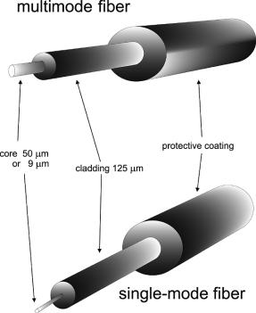
Multimode fibers are characterized by a relatively large diameter of the lightguiding core, which is much larger than the wavelength of the light (Fig. 1.3). In the most common version, the core diameter is 50 μm, embedded in a fiber of 125 μm outside diameter. In contrast, single-mode fibers have a core diameter that is larger than the wavelength only by a small factor; typical values range between 7 and 10 μm. This does not a ect the outer diameter of the fiber, which may be the same as for a multimode fiber; indeed, the outside diameter of 125 μm is the standard value for both fiber types (Fig. 1.4).

Figure 1.3: Multimode fibers and single-mode fibers only di er in the diameter of the light-guiding core, which is made from a glass that is doped in a slightly di erent way than the surrounding cladding.

In first applications, multimode fibers were used. They allow better incoupling e ciency, and there are fewer losses when connecting fibers together. However, as we shall see in Sect. 2.3, single-mode fibers allow higher data rates over longer distances. Therefore, once the connector tolerance issue was solved satisfactorily, single-mode fibers became the favored choice and are almost exclusively used today at least for the long haul. Only for short distances, in particular in local area networks between several computers inside one building, multimode fiber is still preferred because the highest data rate is not required, but some savings can be had in coupling and connecting.

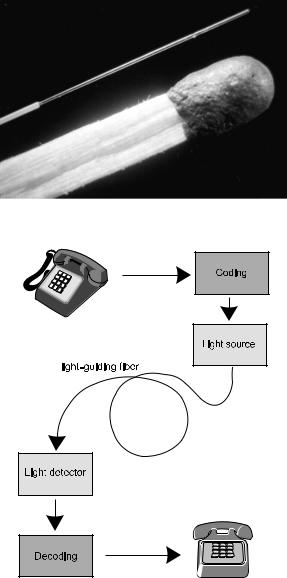
At this point, we should take a look at the basic ingredients of any data transmission system (see Fig. 1.5). The information to be transmitted can originate from a person speaking into a telephone, but it might also come from a telefax machine sending data or from a computer hooked up to a line. In the case

Figure 1.4: A standard optical fiber in comparison to a match.

Figure 1.5: Sketch of a data transmission.

of a human speaker, the acoustic signal is first converted to an electric signal. Then it gets coded to whatever format is appropriate for the transmission.

The coded signal is then passed onto a light source to modulate it. This means that some property of the light wave, for example its amplitude or phase, is influenced by the coded message. The simplest case would be to switch the light source on and o in accordance to a digital signal representing the message.

The modulated light is then sent through the fiber and reaches the receiver where it is decoded and then converted to the required format: In the case of

a telephone, this is a sound wave from the handset; for a telefax, a printout on paper.

Everything would work just fine if transmitter and receiver were sitting next to each other (back to back). The exciting part, and the reason why all this is done at all, is that one can “insert distance” between both stations. One only needs to make sure that over the distance, there are no more than minimal distortions of the signal, so that after decoding the message is still intact and transmission errors are not perceptible. The founder of information theory, Claude Shannon, has mathematically stated the relations between the rate of data transmission, the bandwidth of the line, and the disturbances occurring on the line (see Sect. 11.1.8).

It is important for a successful transmission that the signal is not attenuated too much on the line. As mentioned above, first field trials used visible light, but soon people realized that infrared wavelengths are much better in this respect. One speaks of a first generation of fiber-optic systems that operated around 850 nm, a wavelength that was convenient due to the availability of very economic gallium arsenide laser diodes. This spectral region is also known as the first window for fiber transmission.

The second generation operated at a wavelength around 1300 nm (the second window). This wavelength was favored because the fiber’s dispersion (which is the subject of Chap. 4) is particularly low there. As we shall see, this fact provides a considerable increase of both reach and data rate. The major part of all systems installed today is designed for this wavelength, although emphasis meanwhile shifts to the third window.

The third generation moves on to wavelengths near 1550 nm (the third window). This is the regime where fibers made of fused silica have their global loss minimum (see Chap. 5).

There have been numerous attempts to make fibers such that the main advantage of the second window – low dispersion – would occur at the wavelength of the third window, so that the best of both could be combined. A truly successful implementation would have allowed to phase in the third generation more rapidly. However, while it is possible in principle, the commercial success of these attempts remained limited. One of the reasons that industry preferred to hang on to the second window for a long time was that the installed base of second-generation fiber-optic systems represented a value of billions of dollars; it did not seem to make business sense to give up that legacy. A technical reason also was that fibers with dispersion optimized at 1550 nm turned out to partially lose the advantage of the lowest loss. The strategy today is that di erent fibers are concatenated so that dispersion is partly compensated; we will consider such systems in Sect. 11.2.3.

At this point the reader may ask: Why is it that light in fiber optics is superior to the more conventional electric current over copper cable? The answer to this is found by considering the fundamental limits to transmission losses in comparison with optical fiber and copper wire. For wire it is given by the skin e ect, i.e., the phenomenon that at high frequencies almost all current is carried only in a thin surface layer of a conductor, while the volume contributes little or is even counterproductive. This e ect, as described in Appendix B, increases with frequency and eventually defeats any high data rate, long-distance transmission. Optical fibers do not su er from this limitation and therefore have a clear advantage when it comes to transmitting high data rates over long distances.