

Fiber_Optics_Physics_Technology
.pdf32 |
|
|
|
|
|
|
|
|
|
|
|
|
|
|
|
|
Chapter 3. Treatment with Wave Optics |
||||||||||||
When we now reinsert all terms and multiply with r2/RΦ, we obtain |
|
||||||||||||||||||||||||||||
|
|
|
|
r ∂ |
|
R + |
|
r2 ∂2 |
|
|
|
1 ∂2 |
|
|
|
|
|
|
|||||||||||
|
|
|
|
|
|
|
|
|
|
|
|
|
|
R + |
|
|
|
|
Φ − r2β2 = −k2r2, |
(3.38) |
|||||||||
|
|
|
R |
∂r |
R |
∂r2 |
Φ |
∂φ2 |
|||||||||||||||||||||
which after sorting of terms becomes |
|
|
|
|
|
|
|
|
|
|
|
|
|||||||||||||||||
− |
1 ∂2 |
Φ = |
1 |
r2 |
∂2 |
|
+ r |
∂ |
|
+ r2 |
k2 |
|
β2 |
. |
(3.39) |
||||||||||||||
|
|
|
|
|
|
|
|
|
|
|
|||||||||||||||||||
Φ ∂φ2 |
|
|
∂r R |
− |
|||||||||||||||||||||||||
|
R |
∂r2 R |
|
|
|
|
|
|
R |
|
|||||||||||||||||||
|
|
|
|
|
|
|
|
|
|
|
|
|
|
|
|
|
|
|
|
|
|
|
|
||||||
We see that now the LHS contains Φ and not R; on the RHS it is the other way around. Therefore, both sides must be equal to some constant. We will denote this constant by m2. Now we have two independent equations for the azimuthal and the radial parts of the field amplitude distribution:
|
|
|
|
∂2 |
Φ + m2 |
Φ = 0 |
|
(3.40) |
|
|
|
|
∂φ2 |
|
|||||
|
|
|
|
|
|
|
|||
and |
∂2 |
∂ |
|
|
|
|
|||
|
|
|
|
|
|||||
r2 |
|
R + r |
|
R + r2 k2 − β2 R = Rm2, |
|
||||
∂r2 |
∂r |
|
|||||||
which, by using the abbreviation κ2 = k2 − β2, is written in simpler form as
|
∂2 |
∂ |
|
||
r2 |
|
R + r |
|
R + (κ2r2 − m2)R = 0. |
(3.41) |
∂r2 |
∂r |
||||
To obtain some understanding of the meaning of quantities κ, k, and β, we recall the ray-optical description where we had rays propagating at a small angle with the axis. We assign the propagation constant k to the wave. β was introduced as its component in the propagation direction. Then, one can look at κ as its transverse component.
3.5Modes
The equation for the azimuthal structure, Eq. (3.40), has the general solution
Φ = c0 cos(mφ + φ0) |
(3.42) |
with c0 and φ0 constants. Surely, Φ and ∂Φ/∂φ must be continuous at φ0 and φ0 + 2π. But then, m must be an integer number. This constrains the number of possible solutions of the equation for the radial structure, Eq. (3.41).
Equation (3.41) has the form
x2y + xy + (κ2x2 − m2)y = 0
when one makes the identifications y = R and x = r and interprets the prime as a derivative with respect to x. In this form, or after scaling out κ, the equation is given in mathematical tables. It is called Bessel’s di erential equation. For integer m it is solved by
y = c1Jm(κx) + c2Nm(κx), |
(3.43) |
3.5. Modes |
33 |
whenever κx is real (i.e., κ2x2 ≥ 0), or by |
|
y = c3Im(κx) + c4Km(κx), |
(3.44) |
whenever κx is imaginary (i.e., κ2x2 < 0). Here, functions Jm(κx), Nm(κx), Im(κx), and Km(κx) are Bessel functions. Properties of Bessel functions are given in Appendix C.
In order to find the coe cients c1 to c4, we must finally fix the specific geometry of the fiber. Up to now, we have only assumed cylindrical geometry and a small value of the refractive index di erence. Now we further specify that we consider a step index fiber: This is both a particularly simple structure and a realistic choice. For a step index fiber we have
n = |
nK: |
r ≤ a |
(inside the core), |
(3.45) |
|
nM: |
r > a |
(in the cladding). |
|
Of course, nK > nM because there would be no waveguiding otherwise. In order to distinguish the refractive indices in core and cladding, and also the wave numbers, we will use indices “K” and “M” as in Chap. 2.2. Index “0” continues to denote the respective quantity in vacuum, e.g., kK = nKk0.
In the limiting case when the wavelength is much smaller than the geometric dimensions of the fiber cross-section, we expect to recover the results from ray optics: Light is guided inside the core. Therefore we look for solutions with the dominant part of the light wave concentrated in the core. We conjecture, at the same time, that light in the cladding will have field amplitudes which decrease further away from the center and will at least not contribute dominantly to the guided wave.
But then, κr must be real in the core and imaginary in the cladding. In other words, at least in the core, k ≥ β must hold: The wave number must be larger than or equal to its longitudinal component. In the cladding we may well have the opposite situation. This corresponds to solutions to Bessel’s equation with transversal standing waves in the core and radially decaying waves in the cladding.
We expect on physical reasons that the field amplitude distribution does not have singularities. This implies that for the core the coe cient in the Nm term must vanish. In the cladding, similarly, the coe cient of the Im term must vanish. This makes good physical sense: Far away from the core we expect the field amplitude to decay at least as rapidly as 1/r because otherwise the integral of power over the entire transverse plane would diverge.
In order to have κr real in the core, it is required that at r ≤ a, (κr)2 ≥ 0, or kK2 − β2 r2 ≥ 0. In contrast, in the cladding (i.e., at r > a), we need to have (κr)2 ≤ 0 and thus kM2 − β2 r2 ≤ 0 . Taken together, this implies
kK ≥ β ≥ kM.
The range of possible wave numbers for propagation down the fiber is thus constrained by the requirement of waveguiding.
Once again we introduce abbreviations: The transversal components of the wave number in core and cladding are given by
κK2 |
= |
kK2 − β2, |
κM2 |
= |
− kM2 − β2 ; |
34 |
Chapter 3. Treatment with Wave Optics |
it is customary to use the product of these quantities with the core radius a:
u |
= |
κKa, |
(3.46) |
w |
= |
κMa. |
(3.47) |
u and w are dimensionless, real positive quantities often used in the literature. To comment on their physical significance, su ce it to say that u describes the progression of phase and w the transverse decay of amplitude. One might call u the radial phase constant and w the radial decay constant.
In order to establish a relation between these somewhat abstract quantities and measurable quantities, we use the following relation between u and w:
u2 + w2 = |
kK2 |
− β2 a2 − kM2 − β2 a2 |
(3.48) |
= |
kK2 |
− kM2 a2 |
(3.49) |
= |
k02 nK2 − nM2 a2. |
(3.50) |
|
It is clear that u2 + w2 equals a constant. This constant is of central importance and is called normalized frequency or simply V number. It is given by
V 2 = k02 a2 n2K − n2M
or
V = |
k0 a NA |
|
||||||
|
2π |
|
|
|
(3.51) |
|||
= |
nK2 − nM2 |
|||||||
|
|
a |
|
|||||
|
λ0 |
|||||||
and contains all relevant data of an experimental situation. A step index fiber is characterized by the core radius a and the refractive indices nK and nM or, alternatively, numerical aperture. Either wavelength or vacuum wave number completes the description of the experimental situation. In the following, the value of V will be the decisive criterion to establish how many modes a fiber can support.
Using u and w, the general solution of the wave equation for a step index fiber can be written as:
NK |
= |
CKJm(ur/a) cos(mφ + φ0) : |
r ≤ a, |
|
(3.52) |
NM |
= |
CMKm(wr/a) cos(mφ + φ0) : |
r > a. |
|
|
We recall that from a ray-optical treatment, one would na¨ıvely expect a rectangular field distribution: constant 100% amplitude everywhere in the core and 0% in the cladding. It should by now be obvious that reality is di erent from that.
At r = a both solutions must connect in a smooth way. This means that we do not expect a discontinuity: Rather, we expect the transition to be continuous and di erentiable. This is only possible when the angular dependence is identical for both solutions, which is why in Eq. (3.52) we already wrote the same φ0 and m.
The conditions for smooth transition are
|
|
NK(r = a) |
= |
NM(r = a), |
(3.53) |
||
|
∂ |
|
|
∂ |
|
||
|
|
NK(r = a) |
= |
|
|
NM(r = a). |
(3.54) |
∂r |
∂r |
||||||
3.6. Solutions for m = 0 |
|
|
|
|
|
|
35 |
||||
After inserting, we find |
|
|
|
|
|
|
|
||||
|
|
CKJm(u) |
= CMKm(w), |
(3.55) |
|||||||
CK |
∂ |
Jm(ur/a) r=a |
= |
CM |
∂ |
Km(wr/a) r=a. |
(3.56) |
||||
∂r |
|
|
|||||||||
|
|
|
|
|
∂r |
|
|
||||
In the second of these equations we can introduce |
|
||||||||||
|
|
|
∂ |
= |
u |
|
∂ |
|
|
(3.57) |
|
|
|
|
|
a ∂(ur/a) |
|
||||||
|
|
∂r |
|
|
|||||||
and thus use the argument ur/a throughout; then we can write the derivative at r = a as
C |
|
u |
J |
(u) = C |
|
w |
K |
(w) |
(3.58) |
|
|
|
|||||||
|
K a m |
|
M a m |
|
|
||||
(the prime ( ) denotes the derivative with respect to the argument).
For the existence of a solution, it is required that the determinant of coe -
cients be zero: |
|
|
|
|
|
|
|
|
|
|
|
|
|
|
|
|
|
|
C |
C J |
|
(u) |
w |
K |
(w) |
− |
C |
|
C |
|
K |
|
(w) |
u |
J |
(u) = 0. |
(3.59) |
|
|
|
|
|
|
|||||||||||||
|
K M |
m |
|
a m |
|
|
K |
|
M |
|
m |
|
a m |
|
|
|||
From this, CKCM/a can be eliminated immediately. Now we use a well-known recursion relation between Bessel functions (see Appendix C):
uJ (u) = |
mJ |
m |
(u) |
− |
uJ |
m+1 |
(u), |
(3.60) |
||||||||||||
m |
|
|
|
|
|
|
|
|
|
|
|
|||||||||
wK (w) = |
mK |
m |
(w) |
− |
wK |
m+1 |
(w). |
(3.61) |
||||||||||||
m |
|
|
|
|
|
|
|
|
|
|
||||||||||
With this the derivatives can be eliminated: |
|
|
|
|
|
|
|
|
|
|
||||||||||
Jm(u) mKm(w) − wKm+1(w) |
|
|
= Km(w) mJm(u) − uJm+1(u) |
|
||||||||||||||||
wJm(u)Km+1(w) = uKm(w)Jm+1(u) |
|
|||||||||||||||||||
or |
|
|
|
|
|
|
|
|
|
|
|
|
|
|
|
|
|
|
||
|
|
Jm(u) |
|
|
= |
|
Km(w) |
|
. |
|
|
|
(3.62) |
|||||||
|
|
uJm+1(u) |
|
wKm+1(w) |
|
|
|
|||||||||||||
From this relation between u and w, we will now obtain the permitted solutions for the fundamental mode of the fiber. It is obvious that functions Km(w) on the RHS are always positive while functions Jm(u) on the LHS frequently change their sign. From this, one sees certain combinations of argument values (and thus V numbers) for which solutions are possible.
Explicit solutions are best obtained numerically. However, for our present purpose, we can inspect some special cases which will give us insight without invoking a computer.
3.6Solutions for m = 0
Let us first consider the case of m = 0, which stands for rotationally symmetric field distributions over the fiber’s cross-section. Then the equation is reduced to
J0(u) |
= |
K0(w) |
. |
(3.63) |
uJ1(u) |
|
|||
|
wK1(w) |
|
||
For a survey of possible solutions, we use the following table in which LHS and RHS of Eq. (3.63) are juxtaposed:
36 |
|
|
|
|
|
Chapter 3. Treatment with Wave Optics |
||||
|
|
|
|
|
|
|
|
|
|
|
|
u |
J0 |
J1 |
J0/uJ1 |
|
K0/wK1 |
|
w |
|
|
0 |
1 |
0 |
∞ |
|
∞ |
|
0 |
|
|
|
. |
|
|
|
|
|
|
|
|
|
|
. |
+ |
+ |
+ |
|
+ |
|
+ |
Branch of solutions |
||
. |
||||||||||
2.405 |
0 |
+ |
0 |
|
0 |
∞ |
|
|
||
. |
|
|
|
|
|
|
|
|
|
|
. |
− |
+ |
− |
|
− |
|
− |
No solution |
||
. |
||||||||||
3.832 |
− |
0 |
∞ |
|
∞ |
|
0 |
|
|
|
. |
|
|
|
|
|
|
|
|
|
|
. |
− |
− |
+ |
|
+ |
|
+ |
Branch of solutions |
||
. |
||||||||||
5.520 |
0 |
− |
0 |
|
0 |
∞ |
|
|
||
. |
|
|
|
|
|
|
|
|
|
|
. |
+ |
− |
− |
|
− |
|
− |
No solution |
|
|
|
. |
|||||||||
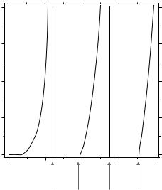
There is an alternation of ranges with and without solutions. The table only checks the algebraic sign; we can go beyond that and actually compute the values pertaining to the branches of solutions and plot them in a diagram of the (u, w) plane. This is done in Fig. 3.1. The curves represent ratios of two Bessel functions; their shape looks similar to a plot of a tan function. This is not surprising as we state in Appendix C that J0 resembles a cosine function and J1 a sine function.
w
8
01 |
02 |
03 |
6
4
2
0
0 |
2 |
4 |
6 |
8 |
u
2.405 3.832 5.520 7.016
Figure 3.1: Solutions of the eigenvalue equation for m = 0 in the u–w plane. As u increases, there is an alternation between regimes with existing (e.g., 0 ≤ u ≤ 2.405) or nonexisting (e.g., 2.405 ≤ u ≤ 3.832) solutions. Labels at the branches denote indices mp of the LPmp modes, as explained in Sect. 3.9.
Additionally, we can plot the locus of all points pertaining to a given V number. They form segments of circles in the (u, w) plane. For a given fiber, circles with di erent radii correspond to experiments at di erent wavelengths. The

3.7. Solutions for m = 1 |
37 |
other way to look at it is that for a given wavelength, di erent radii correspond to di erent core diameters.
Points of intersection between the tan-like branches with the circle segments define possible solutions, i.e., combinations of u and w in a particular given situation (V fixed). Obviously the first branch of solutions exists at any V number between zero and infinity. The second branch shown here exists only above a minimum V . It takes the value of V = 3.832, as given by the first zero of Bessel function J1. For all other branches shown one can make a similar statement about the minimum V which is always defined by a zero of J1.
3.7Solutions for m = 1
We might proceed by directly inserting m = 1 into the eigenvalue equation Eq. (3.59). This is not a problem for a computer solution. However, here we want to get a feel for the situation without recourse to a computer, and therefore it is advantageous to use an alternative recursion relation of Bessel functions which contains not m + 1 but m −1. This way we obtain an equation for m = 1 which again only contains J0 and J1 (instead of J1 and J2); this makes our argument more transparent.
So let us use
uJm(u) = −mJm(u) − uJm−1(u) and wKm(w) = −mKm(w) − wKm−1(w)
in Eq. (3.59) to obtain
− J1(u) = K1(w) . uJ0(u) wK0(w)
In precise analogy to the procedure shown above we can again write a table to locate the possible branches of solutions:
u |
J1 |
J0 |
−J1/uJ0 |
|
K1/wK0 |
|
w |
|
0 |
0 |
1 |
0 |
|
0 |
−∞ |
No solution |
|
. |
|
|
|
|
|
|
|
|
. |
+ |
+ |
− |
|
− |
|
− |
|
. |
|
|||||||
2.405 |
+ |
0 |
−∞ |
|
−∞ |
|
0 |
|
. |
|
|
|
|
|
|
|
|
. |
+ |
− |
+ |
|
+ |
|
+ |
Branch of solutions |
. |
||||||||
3.832 |
0 |
− |
0 |
|
0 |
|
∞ |
|
. |
|
|
|
|
|
|
|
|
. |
− |
− |
− |
|
− |
|
− |
No solution |
. |
||||||||
5.520 |
− |
0 |
−∞ |
|
−∞ |
|
0 |
Branch of solutions |
. |
|
|
|
|
|
|
|
|
. |
− |
+ |
+ |
|
+ |
|
+ |
|
. |
|
|||||||
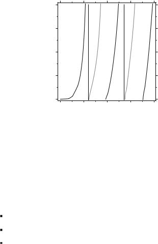
Again we find an alternation between permitted and forbidden regimes, with the changes occurring at zeroes of Bessel functions. In comparison to m = 0, here the regimes switch roles. This way there is a branch of solutions beginning at V = 2.405, constituting a second mode beyond the fundamental mode. Figure 3.2 combines all solutions found so far, i.e., for m = 0 and m = 1.
38 |
Chapter 3. Treatment with Wave Optics |
w
8
01 11 02 12 03
6
4
2
0
0 |
2 |
4 |
6 |
8 |
u
Figure 3.2: Solutions of the eigenvalue equation for m = 0 and m = 1 in the u–w plane for m = 1. Now there are branches of solutions where there were gaps in Fig. 3.1.
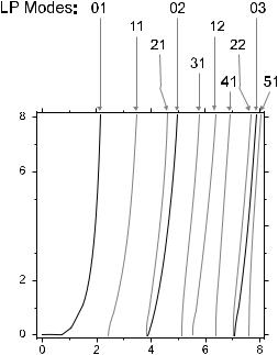
3.8Solutions for m > 1
At larger m values one again finds that allowed and forbidden ranges alternate, with the transitions occurring where V equals zeroes of Bessel functions. Figure 3.3 shows all modes up to V = 8.
We wrap up what we have learned:
For V < 2.405, there is only one branch of solution.
For V ≥ 2.405, there are initially two branches.
At certain still higher V values, more branches come up.
The particular value V = 2.405 marks the transition from the existence of a unique solution to more than one solutions. Below, the fiber is said to be single-moded. This first mode is called the fundamental mode, the transition point is the cuto of higher-order modes. For any given fiber, one can calculate the corresponding cuto frequency or wavelength from V = 2.405. At lower frequencies (longer wavelengths) the fiber is single-moded. This implies that some fiber is not single-moded in an absolute sense: Such statement has meaning only in relation to a specified wavelength.
3.9Field Amplitude Distribution of the Modes
We now see that the modes form a two-parameter family. One of the parameters is m. m indicates the angular dependence of the field distribution of the mode. For m = 0 the distribution is rotationally invariant, i.e., on any circular path around the center one would find a constant field amplitude (and thus intensity). For m = 1, the field amplitude will vary according to a sine function of the azimuthal angle. It therefore has two zeroes at mutually opposite positions;
3.9. Field Amplitude Distribution of the Modes |
39 |
w

u
Figure 3.3: All solutions of the eigenvalue equation in the u–v plane up to u, w = 8.
in between there are a positive and a negative branch, or lobe. Either branch contains a maximum of the intensity while the algebraic sign indicates the phase of the field. Thus, in one lobe the field oscillates in opposite phase to the other. For m = 2, a circular path would run through two full periods of the sine function; the intensity pattern then resembles a four-leafed clover. Again, each pair of leaves in opposite positions has the same phase while the other pair has opposite phase. When m takes even higher values, the angular dependence of the intensity has 2m leaves.
m also fixes which Bessel functions govern the field distribution in radial direction: We have found a combination of Jm in the core and Km in the cladding. Since Jm oscillates (at any m), there are infinitely many ways to smoothly connect Jm to Km even after m has been fixed. (Recall that the signs of coe cients CM and CK in Eq. (3.52) were arbitrary). This set of possibilities is labeled with p, the second parameter. We adopt here the terminology of modes as introduced in 1971 by Gloge [50]: Modes are designated with “LPmp” on grounds that they are essentially linearly polarized. Index m designates the number of pairs of nodes in the azimuthal coordinate, and index p counts the possibilities in the radial coordinate.
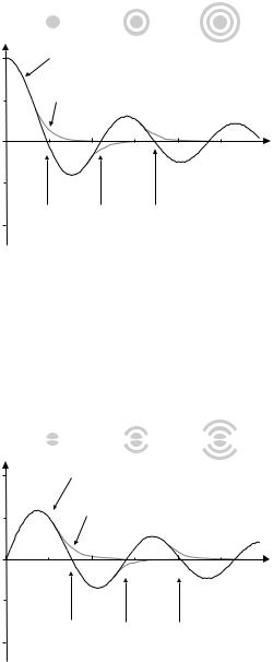
We can now sketch what the intensity distribution of the modes looks like. Figures 3.4–3.6 show the various possibilities to make the connection between the Jm and Km terms and give an idea about the intensity distribution.
40 |
Chapter 3. Treatment with Wave Optics |
LP01 |
LP02 |
LP03 |
1 |
J0 |
K0
0
5 10 ur/a
p = 1 p = 2 p = 3
– 1
Figure 3.4: Construction of the radial intensity distribution for modes with m = 0.
LP11 |
LP12 |
LP13 |
1 |
J1 |
|
K1
0
5 10 ur/a
p = 1 p = 2 p = 3
– 1
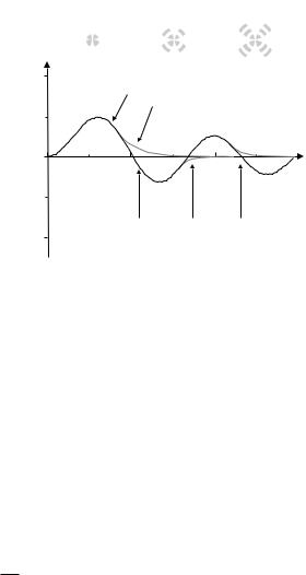
Figure 3.5: Construction of the radial intensity distribution for modes with m = 1.
3.10. Numerical Example |
|
41 |
LP21 |
LP22 |
LP23 |
1 |
|
|
J2 |
K2 |
|
|
|
|
0 |
10 |
ur/a |
5 |
||
p=1 |
p= 2 |
p= 3 |
–1 |
|
|
Figure 3.6: Construction of the radial intensity distribution for modes with m = 2.
Between V = 0 and V = 2.405, there only exists the branch of solution pertaining to the LP01 mode. This is called the fundamental mode of the fiber; it has a particularly simple shape, not unlike a bell shape. Between V = 3.832 and V = 5.520 we additionally find the LP02 mode. As V increases, new modes keep coming up.
This reasoning is borne out very well by experimental observation. In [145], all modes were excited separately so that the intensity pattern at the fiber end could be photographed individually. Figure 3.7 shows the result.
3.10Numerical Example
We consider a typical numerical example to illustrate the transition from a single-mode fiber to a multi-mode fiber. Take a fiber with a = 4 μm, =
3 × 10⁻³, and n = 1.46 . From the definition of V , using the approximation
√ K
NA = nK 2Δ, and the cuto condition V = 2.405, one immediately obtains the condition for the cuto wavelength:
|
√ |
|
|
|
λcuto = |
2π a nK 2Δ |
. |
(3.64) |
|
|
||||
|
2.405 |
|
|
|
Inserting the numbers, we obtain λcuto = 1.182 μm. This fiber is then a singlemode fiber for all wavelengths longer than 1.182 μm. This includes the 1.3- and 1.55-μm range preferred in telecommunication. For wavelengths shorter than λcuto there is more than one mode: A second mode appears at this cuto , and at some particular even shorter wavelength yet another mode appears. This wavelength is obtained from the same condition by simply replacing V = 2.405 with V = 3.832. One obtains 742 nm.
For even larger V (even shorter wavelengths) more and more modes are added. The same fiber which supports just a single mode in the infrared will carry several modes in the visible! As V grows very large, the wavelength