Fiber_Optics_Physics_Technology

Figure 4.14: Schematic refractive index profile of a quadruple-clad fiber. Here five indices and four radii must be distinguished.

Figure 4.15: Pseudo-3D rendering of a quadruple-clad fiber profile. From [102].

1.2 1.5

Figure 4.16: Tailoring of the dispersion curve through choice of suitable index profiles: dispersion-shifted and dispersion-flattened fiber in comparison to a standard step index fiber.

The motivation to tailor the dispersion curve is to get the best of two worlds: the minimal dispersion of the second window combined with the minimal loss in the third window. Dispersion flattened fibers have low dispersion at both the second and third windows at the same time; such fibers can be used as direct replacement for older fiber designed for the second window but provide the added benefit of also performing well in the third window.

4.6Polarization Mode Dispersion

Up to now we have disregarded the fact that a light field is fully characterized only when one takes its state of polarization into account. Di erent states of polarization propagate di erently, thus arises a special type of dispersion which we now examine closer.

As we derived the modal profiles in Chap. 3, we used the approximation of a homogeneous material and found that all modes are twofold degenerate into distinct orthogonal linear polarization states. The approximation is valid only, of course, when there is weak guiding (Δ very small). In the more general case the modes are not exactly linearly polarized, because the index discontinuity at the core–cladding interface distorts the modal structure. Nonetheless, the approximation can be useful.

Moreover, we had assumed isotropy. This implies that the orientation of the two planes of polarization is arbitrary. One might then conclude that launching linear polarized light at any orientation will produce light of the same linear polarization at the fiber end. This is not what experience shows.

In any real fiber there is some – potentially very weak – deviation from ideal circular symmetry. We have to distinguish between (a) geometric deviations, like when the core is asymmetric or not centered well; (b) optical deviations like when the material index is not homogenous; and (c) mechanical deviations due to stress-induced birefringence. The latter contribution may arise either due to tension built into the fiber – after all, the fiber is rapidly cooled during its manufacturing which may well introduce tension – or due to tension created during use as the fiber is being bent.

All these deviations from perfect circular symmetry conspire to create differences for the propagation of the two polarization modes. This gives rise to polarization mode dispersion. We will now consider how it manifests itself and how to avoid it.

4.6.1Quantifying Polarization Mode Dispersion

Rather than a single propagation constant β we now need to use two, βx and βy , to describe conditions for the two polarization states linearly polarized in x and y directions. As soon as βx = βy , the two light waves polarized in parallel to x and y will propagate di erently; hence, they will be alternatingly in phase and out of phase with each other. This occurs with spatial period

Figure 4.17: Several polarization-maintaining structures. In each case the circular symmetry is broken.

Y

2D Refractive index profile of bowtie fiber. Y

Figure 4.18: Pseudo-3D rendering of the refractive index profile for a bowtie fiber. With kind permission from Fibercore [9].

Such geometries allow B = 3 to 8 × 10−4 corresponding to Λ = 1 to 3 mm. The beat length is thus reduced by three orders of magnitude and is now shorter than the tightest possible bend radii. Therefore, the built-in birefringence due to this structure overwhelms the random birefringence including any that may occur during operation due to bending. Why is this, then, a polarizationmaintaining fiber?

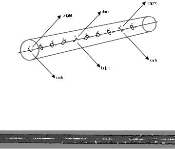
If one launches light which is linearly polarized along the direction of one of the two axes of the elliptical structure, this state of polarization will be maintained. If, however, the light is polarized at an angle with the axes, one can mentally decompose it into the two parts along the axes: These will propagate with di erent velocity because they experience a di erent refractive index. The state of polarization will then cyclically evolve through linear → elliptic → circular → elliptic again → linear again, etc. This evolution can be exploited to measure the beat length in a particularly simple experiment: The weak scattered light exiting the fiber sideways appears modulated with a spatial period because dipoles do not radiate energy in the direction along their own axis (see Figs. 4.19 and 4.20).

How well does a polarization-maintaining fiber actually maintain the state of polarization? This is quantified by the extinction ratio E, defined as

Here, indices p and s distinguish the fractions of power P which are polarized parallel (p) or perpendicular (s, as in German senkrecht) to the initial polarization plane.

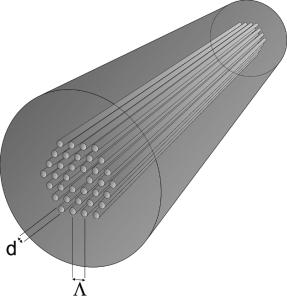
Figure 4.21: A schematic view of a typical holey fiber. Tubular channels run along the entire length of the fiber parallel to the core which they surround in a certain geometric arrangement. The hole diameter d and pattern pitch Λ are indicated. In the case shown here, the core is at the position of the “missing” channel at the center.

the fiber so that a pattern of holes appears in the cross section (see Fig. 4.21). Manufacturing of these fibers di ers from the conventional procedure as described in Sect. 6.2: The preforms are produced by stacking together a bunch of glass tubes; that stack is then fused together and drawn into a fiber. This is often done in two steps: fusing into a “cane” as an intermediate, then the final drawing into a fiber. The drawing process is modified to proceed at a somewhat slower speed and at lower temperature so that the holes do not collapse.

The array of holes in the cladding gives rise to the (somewhat tongue-in- cheek) name of “holey” fibers. The air-filled holes reduce the e ective index of the cladding so that dopants to raise the core index are not normally applied: The index di erence can easily exceed the 1% limit maximally obtainable with dopants by far. The regularity of the hole pattern is not crucial in this type of microstructured fibers; in fact, even fibers with random hole arrangements have been demonstrated [117].

On the other hand, a strictly periodic arrangement with a pitch not much di erent from the wavelength of the light can give rise to resonant reflectivity when a certain Bragg condition is met; this is very reminiscent to e ects with X- rays passing through crystals (actually, this is how we know the size of crystal cells) and thus gives rise to the name of photonic crystal fibers. There is an actual distinction between these two fiber types, but as of this writing, the names are not used very consistently in the community. We will here adopt the following definitions:

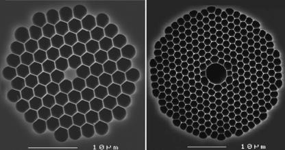
Holey fiber designates a microstructured fiber with hollow channels surrounding the core which itself, however, is massive.

Photonic crystal fiber designates a microstructured fiber with hollow channels surrounding the core which is also hollow.

Figure. 4.22 shows examples of both types in comparison. We will briefly outline both types and point out their remarkable properties which cannot be had from conventional (massive) fiber and which open up exciting possibilities for novel applications. See also Fig. 4.23.

Figure 4.22: Comparison of two basic types of microstructured fibers. In both cases a central region around the core is shown. Left : Holey fiber (Type NL-24- 800). Right : Photonic crystal fiber (Type HC-633-01). Both fibers are manufactured by Crystal Fibre AS. With kind permission by NKT Photonics, Birkerød, Denmark.

4.7.1Holey Fibers

In conventional fibers, there is a core which by way of suitable doping has a somewhat higher refractive index than the cladding which surrounds it. Due to constraints in the chemistry, the index di erence can be no larger than about 1%. In holey fibers, the cladding has a sizeable air fraction so that its e ective index is lowered. These fibers are also known as solid-core photonic crystal fibers.

The light wave experiences an index which has contributions from both the air holes and the remaining glass in between. In the case of a regular hole pattern, one can distinguish two quantities: the hole diameter d and the pitch Λ. These are often combined with the wavelength of the light into the normalized hole diameter d/Λ and the normalized spatial frequency Λ/λ. A precise calculation of the e ective index and the modal structure requires numerical procedures which can be quite involved. It is straightforward, though, to see the following.

The void content lowers the e ective index with respect to that of the glass. The e ective cladding index is therefore a function of the air fill fraction AFF,

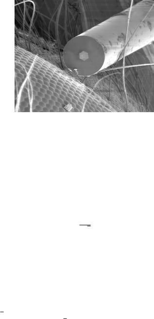
Figure 4.23: A holey fiber seen in an electron microscope together with the eye of an ant. Insects are endowed by nature with a regularly patterned eye. The structure of a holey fiber follows a similar design. The author thanks Toralf Ziems for his assistance in taking this picture.

the ratio of air channel volume to total cladding volume. For the hexagonal geometry shown in Fig. 4.21 it is calculated by straightforward geometry as

This expression, by the way, tells us that as the holes get bigger to the point that the glass walls in between vanish at d = Λ, the air-filling fraction is bounded by

π

AFFmax = √ = 0.9069 . 2 3

When the wavelength is shorter than both the pattern pitch and the hole size, light will be guided primarily by the glass bridges between the holes. This suggests that in the limit of λ → 0 the e ective index tends to that of the glass alone. When on the other hand the wavelength is much larger than the structural dimensions, the light field cannot ‘feel’ the holes and interstitial glass separately. The e ective index may then be expected to be some suitably weighted average of the indices of glass and air. This is the reason for a strong dependence of e ective cladding index on wavelength.

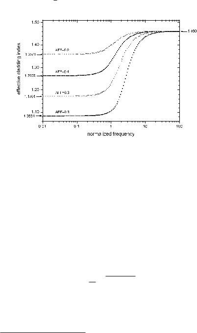
The situation is demonstrated in Fig. 4.24 which shows the e ective cladding index for an infinite triangular array as a function of normalized optical frequency ν = νΛ/c for four di erent air fill fractions. The normalization was chosen so that conveniently at ν = 1 the (vacuum) wavelength coincides with the pattern pitch. The glass index was here assumed to be at a constant nglass = 1.4600, and that of air at nair = 1, to avoid a complication of the present discussion by issues of material dispersion. Data points were calculated using the freely available software described in [79].

For very high frequencies the e ective index tends to that of the glass as expected (arrow at right axis). For very low frequencies the e ective index

N ,

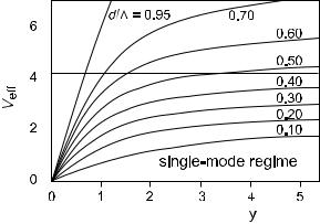
Figure 4.25: V number in a holey fiber as a function of normalized frequency Λ/λ. The parameter is d/Λ. Toward high frequencies, Ve tends to some constant. It never crosses the cuto (marked by horizontal dotted line) as long as d/Λ < 0.4. Then the fiber supports only one mode at any frequency. After [29].

i.e., the fundamental mode that would occupy an infinitely extended cladding pattern without the central defect which is the core.

As pointed out above, nFSM tends to the material index as frequency increases. This partially cancels the λ term in the denominator so that V is not proportional to frequency but rather becomes almost constant at Λ/λ 1, with the specific value depending on d/Λ (see Fig. 4.25).

Through this e ect one obtains a remarkable property which is called the endlessly single-mode property [28]. It has been found that for d/Λ small enough (more precisely: d/Λ < 0.406 [91]), there is only one mode supported at any frequency. This means that within the practical limits set by wavelengthdependent loss, the fiber is always a single-mode fiber. This has been verified over a tremendous frequency range of e cient waveguiding, which may run from ultraviolet to infrared – a factor of 4 [28].

Holey fibers have a second very remarkable property, and this regards their dispersion behavior. For small air-filling fractions, the influence of the holes is small and the wavelength dependence of group velocity dispersion can be expected to closely follow the material dispersion. This is indeed the case. However, as the hole size increases, there is a growing contribution from waveguide dispersion which can reach the point of overwhelming material dispersion. Since the waveguide contribution can be anomalous at short wavelengths, the zerodispersion wavelength can shift toward shorter wavelengths. The reader will recall that this is not possible with conventional fiber. At about d/Λ = 0.30, dispersion is flattened over a sizable interval. The precise wavelength range of this interval can be shifted by adjusting the pitch size Λ. Fibers are being o ered commercially where this range begins at about 1 μm or even 800 nm. Finally, by judicious choice of pitch and hole size, the dispersion can be even made to have a maximum in this spectral range so that there can be two zero-dispersion wavelengths, similar to the case of the dispersion-flattened conventional fiber