

Fiber_Optics_Physics_Technology
.pdf208 |
Chapter 10. A Survey of Nonlinear Processes |
do not get perturbed by it. They exist at anomalous dispersion; it is fortunate that the wavelength regime of anomalous dispersion in fiber coincides with the wavelength regime of lowest losses. This is why solitons lend themselves to applications in long-haul data transmission. Chapter 11 is devoted to a more detailed discussion of this aspect.

Part V
Technological Applications
of Optical Fibers
Laying optical fiber cables – here within sight of the author’s house – is not nearly as spectacular as the performance of fiber during operation.

Chapter 11
Applications in
Telecommunications
11.1Fundamentals of Radio Systems Engineering
We first present a brief introduction to essential concepts of telecommunications engineering, insofar as they are relevant for our topic.
11.1.1Signals
The central concept of all communication engineering is that of a signal. In the most general case, it is left open what this is physically; it su ces to state that it is a scalar, real-valued function of time. We assume that the signal contains information which is meant to be taken from some transmitter to some receiver. The signal may be represented by some physical quantity such as an electric voltage, the position of an indicator needle, or the brightness of a light source; one common realization would be that at each instant, the value of the quantity is proportional to that moment’s value of the signal.
We must first distinguish continuous-time signals and discrete-time signals. The latter have a defined value only at certain instants in time, or in other, more mathematical words consist of a sequence of Dirac pulses (delta functions), each weighted in accord with the signal value. One can obtain a discrete-time signal from a continuous-time signal by sampling. Very frequently one chooses to take samples at a fixed rate, i.e., in equal time steps. Below we will assume a fixed sampling rate, or clock frequency, throughout.
The other fundamental distinction is between analog signals and digital signals. An analog signal has a continuous range of values, i.e., can take any intermediate value within the interval of possible values. In contrast, a digital signal has a finite number of possible states known as its alphabet.
A thermocouple yields a voltage proportional to temperature; this is an example for an analog continuous-time signal. A dynamic microphone is another example of the same. A sequence of results when dice are thrown or the roulette wheel is turned would represent a discrete-time digital signal. Is is quite often the case that digital signals are also discrete-time.
F. Mitschke, Fiber Optics, DOI 10.1007/978-3-642-03703-0 11, |
211 |
c Springer-Verlag Berlin Heidelberg 2009
212 |
Chapter 11. Applications in Telecommunications |
An important subclass of digital signals are binary signals. For these the alphabet has just two symbols which, depending on context, may be called “zero” and “one”, “high” and “low”, “true” and “false”, or “plus” and “minus”, etc.
11.1.2Modulation
Only in the simplest cases a signal is transmitted just as is. There are many benefits if one uses a carrier oscillation, a wave on which the signal is “impressed”. This is familiar from broadcast signals: At the receiver one selects the carrier frequency of the desired program. This way several di erent programs can be transmitted simultaneously and independently.
The impression of a signal onto a carrier is known as modulation. It can be done in a variety of ways: If the carrier is a harmonic periodic function (this is a very common situation), which can be written as
A = A0 cos(Ωt + ϕ) |
(11.1) |
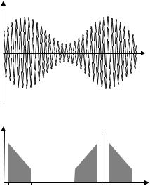
with amplitude A0 and angular frequency Ω, one has the options of subjecting either A0, Ω, or ϕ to the signal. The result is then referred to as amplitude modulation, frequency modulation, or phase modulation, respectively.
Amplitude Modulation
Let us assume for simplicity that the range of values of the signal S(t) is restricted to the interval −1 ≤ S(t) ≤ +1. This can always be achieved by proper normalization. One can then make the amplitude signal-dependent by letting
ˆ
A0 = A (1 + S(t)) in Eq. (11.1) to obtain amplitude modulation (Fig. 11.1). Again for the sake of simplicity, we consider the simplest possible signal, a
sinusoidal oscillation with angular frequency ω:
S(t) = sin ωt. |
(11.2) |
|
ˆ |
≤ M ≤ 1 is called modulation depth. |
|
We now let A0 = A (1 + M sin ωt) where 0 |
||
We insert in Eq. (11.1) and obtain
ˆ
A = A (1 + M sin ωt) cos(Ωt + ϕ).
Using the well-known relation between harmonic functions
|
|
1 |
sin(x − y) + sin(x + y) , |
|
|
|||
sin x cos y = |
|
|
|
|||||
2 |
|
|
||||||
this then yields |
|
|
|
|
|
|
|
|
A = Aˆ cos(Ωt + ϕ) + M sin ωt cos(Ωt + ϕ) |
|
|
|
|
||||
= Aˆ cos(Ωt + ϕ) + |
M |
sin(ωt + Ωt + ϕ) + sin(ωt |
− |
Ωt |
− |
ϕ) |
||
|
||||||||
2 |
|
|
|
|
|
|||
(11.3)
(11.4)
This result contains terms of three di erent frequencies: The first term on the RHS at Ω corresponds to the carrier. The second and third terms have frequencies Ω ± ω. Amplitude modulation (AM) generates new frequency components: the one at the carrier frequency persists, and one each above and below the carrier frequency by a di erence equal to the signal frequency are new.
11.1. Fundamentals of Radio Systems Engineering |
213 |
Field amplitude
Time |
Spectral |
carrier |
|
power density |
||
|
ωmin ωmax |
Ω |
Frequency |
base band |
lower |
upper |
|
sideband |
|
Figure 11.1: Sketch to explain amplitude modulation. Top: The modulation of a carrier wave with frequency Ω with a signal ω = 0.05 Ω is shown at a modulation depth of M = 0.5. Bottom: Modulation generates two sidebands above and below the carrier, at the distance of the signal frequency. The figure suggests a signal occupying the band ωmin ≤ ω ≤ ωmax (baseband). The sidebands have the same width. Note that the lower sideband is inverted.
Fourier components with a frequency equal to carrier frequency plus signal frequency are collectively called the upper sideband; those at carrier frequency minus signal frequency, lower sideband. For our example of a sinusoidal modulation, these “bands” consist of only one sharply defined frequency. However, any realistic signal will be more complex than that of Eq. (11.2), and may be decomposed by Fourier analysis into harmonic functions within a certain spectral interval. Only then are the sidebands aptly named, when we adopt the usage of the term “band” in the sense of “frequency interval.” The di erence between the highest and the lowest frequency occurring in the signal is the bandwidth. The bandwidth of a signal is arguably its most important characteristic and will concern us below.
In the spectrum of the amplitude modulated signal, the upper sideband is a replica of the original signal spectrum, translated in frequency space by the carrier frequency. The lower sideband is a shifted and inverted replica.
The combination of carrier and two sidebands is a rather redundant representation of the signal. Each sideband contains the same information; the carrier, none. Much of the transmitted energy is thus wasted to the carrier. This is why engineers have come up with variants to amplitude modulation in which one sideband and the carrier are suppressed for the transmission. This is called single sideband, or SSB, transmission. It is routinely used in commercial
214 |
Chapter 11. Applications in Telecommunications |
radio transmission because it carries the same amount of information at much lower radiated power, and occupies only half of the bandwidth. For broadcasting purposes, however, SSB is not used because the receivers to decode SSB are slightly more complex.
Angle Modulation
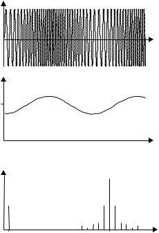
Instead of imposing the signal onto the amplitude in Eq. (11.1), one can make either Ω or ϕ signal dependent. (Of the three quantities, two remain constant in each case). Then one obtains frequency or phase modulation, respectively (Fig. 11.2). In both cases it is the phase angle of the carrier which is acted upon, so that both cases are collectively called angle modulation. Mathematically, in both cases, there is a term of the form
sin (a + b sin(Ωt)) (a, b are constants), |
(11.5) |
and “sine of sine” produces Bessel functions (see Appendix C).
Angle modulation creates sidebands, too. The di erence is that even in the case of a purely sinusoidal signal, more than a single Fourier component appears
Field amplitude
Time
Instantaneous frequency
Ω
Time
Spectral
carrier
power density
ω |
|
Ω |
Frequency |
base band |
lower |
|
upper |
|
|
side bands
Figure 11.2: Frequency modulation. Top: The modulated oscillation in the time domain. Center : The instantaneous frequency follows the signal. Bottom: Several sidebands are generated both above and below the carrier.
11.1. Fundamentals of Radio Systems Engineering |
215 |
both above and below the carrier. Their frequency di erences from the carrier are equal to integer multiples of the signal frequency; their amplitudes can be evaluated using said Bessel functions. We will not pursue this context any further here; instead, the interested reader is referred to texts on communications engineering (e.g., [129]).
Intensity Modulation
The types of modulation described so far are applicable when a monochromatic carrier wave is available. In the realm of optics, only lasers can provide monochromatic waves or an approximation thereof.
Unfortunately, in most cases, it is not guaranteed that the laser emission is truly single frequency. This is certainly not the case for lasers operating on several modes simultaneously. Not all types of lasers can easily be operated in a single mode, and for many laser types used in optical telecommunications this is indeed di cult to achieve. If, however, a laser operates on a multitude of modes simultaneously, the modulation formats described above are not applicable.
Moreover: even when a laser runs in single-mode operation, strictly speaking the oscillation is not monochromatic. Rather, it covers a narrow frequency band (the emission line width) which may be small compared to optical frequencies, but at the same time may be larger than typical signal frequencies. The emission line width of a single-mode laser is determined by several factors. These include technical considerations such as fluctuations of parameters (vibration of components, temperature fluctuations, etc.); these may be removed in principle, but practically speaking that is a very di cult task. But then there are also fundamental limits as set by spontaneous emission in the laser medium. Each emission act brings about a perturbation of the phase of the light wave. As a result there is a finite (nonzero) line width, which was first described by A. Schawlow and C. Townes, pioneers of laser physics [174]. In real-world lasers, the Schawlow–Townes limit may be very low, indeed in the millihertz regime so that it is always swamped by technical perturbations which typically are several orders of magnitude larger. But the same reasoning also implies that there is always – by principle – a phase modulation present in the emission of even the technically perfect laser, and it is a modulation by a random signal. For demodulation (decoding) of phase modulation one needs a reference phase, and in the context of lasers and optics that is always di cult to have. It is true, of course, that oscillators in radio frequency engineering in principle su er from the same line width limit. However, in the radio frequency range, the energy of the quanta, which is proportional to frequency, is so much lower as to be perfectly negligible.
All di culties related to the spectral content of the carrier can be avoided by using intensity modulation. In this technique, one controls the total intensity in the same way as kids playing with flashlamps and sending each other Morse signals. This can be done for light sources with any spectral composition.
Intensity modulation is very simple and is widely used. It can be achieved for laser diodes or luminescent diodes (LEDs) by simply modulating the operational current. This also produces an additional frequency modulation because changes in current produce temperature changes in the chip, but that is irrelevant as long as spectral information is not evaluated.

216 |
Chapter 11. Applications in Telecommunications |
Applications which demand the highest data rates and/or longest distances of transmission are sensitive to dispersion and thus to spectral composition. In such cases single-mode lasers (e.g., of the distributed Bragg type, see Sect. 8.9.3) are preferred light sources; in the interest of keeping the emission frequency stable, one keeps the current constant and applies the modulation with an external modulator.
11.1.3Sampling
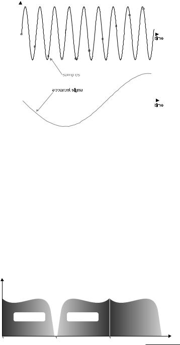
Digital transmission formats are today by far the most successful formats. The signal to be transmitted is digitized, i.e., reduced to a finite number of values in the process of sampling , almost always at a certain fixed rate, the sampling rate. Speaking in mathematical terms, the original signal is multiplied with a periodic sequence of delta functions (a “picket fence”). The continuous signal is thereby replaced with a sequence of delta functions with weight factors corresponding to the respective signal value. This must be done in such a way that the relevant information contained in the signal is represented by the sequence.
It is therefore important to select a suitable sampling frequency. It should be obvious that the sampling frequency must be higher than the highest signal frequency of interest; one can hardly represent an oscillation with fewer sample points per period than just one. If the sampling rate is too low, another complication arises: Fig. 11.3 demonstrates that in the sampling process, certain new frequency components are generated which were not present in the original signal. The reason is that the sequence of delta functions can create beat notes with Fourier components of the signal,1 so that di erence frequencies between sampling frequency and some signal frequencies appear. These undesired additions to the signal are called aliasing signals.
Aliasing signals are, of course, highly undesirable because they prevent a faithful reconstruction of the original signal at the receiving station. They can be avoided by the following precautions:
1.The signal bandwidth is strictly limited with steep-slope low-pass filters to a certain maximum frequency. For this limit, one selects the highest frequency deemed necessary for the transmission in terms of reproduction
quality. For high-fidelity music formats as used for CD recording, this limit is chosen as 20 kHz, i.e., the highest frequency audible to a human ear under the most favorable circumstances. For telephone signals one chooses 4 kHz as the highest frequency (the low-pass filter begins to roll o slightly below that because “brick wall” filters do not exist) because that is su cient for a good intelligibility of the spoken word.
2.Then the sampling frequency is fixed according to the sampling theorem [172], which stipulates that it must be at least twice the highest signal frequency. This way it is guaranteed that no overlap exists between signal band and alias band (see Fig.11.4). For high-fidelity music signals as on CD the sampling frequency is chosen as 44.1 kHz, and for telephone signals, 8 kHz.
1According to the convolution theorem of Fourier transforms, the spectrum of the sampled signal is found as the product of the spectra of original signal and picket fence. It contains the infinite series of harmonics from the sequence of delta functions, each with an upper and lower sideband from all Fourier components of the signal.
11.1. Fundamentals of Radio Systems Engineering |
217 |
|||
|
|
|
|
|
|
|
|
|
|
|
|
|
|
|
|
|
|
|
|
|
|
|
|
|
|
|
|
|
|
|
|
|
|
|
|
|
|
|
|
Figure 11.3: If the sampling rate is only marginally larger than the signal frequency, a beat note at the di erence frequency appears in the sampled data. This spurious contribution is called aliasing signal.
Each sample is then represented after analog-to-digital conversion by a binary number with a given number of digits. More digits give more faithful amplitude resolution but are more costly to transmit. Therefore the number of digits (the “bit resolution”) is dictated by the required quality of transmission. For high-fidelity music, one takes at least 16 bits or one value out of 65,536; in studio recording 24 bits is now standard. For telephone signals 8 bits (one value out of 256) is deemed good enough because it already provides quite good intelligibility.
In this way, the original signal is represented by a stream of binary digits, i.e., zeroes and ones. They represent a discrete-time, discrete-amplitude version of the signal. The bit rate is obtained from sampling rate and bit resolution. For sampling with 8 kHz and at 8 bits resolution one has 64 kbit/s; during each
Spectral power density
signal |
|
alias signal |
|
|
0 |
0.5 |
|
|
|
1.0 |
Frequency |
|||
Sample frequency
Figure 11.4: Beat notes between Fourier components of the signal and the sampling frequency generate sidebands to the sampling frequency called aliasing bands. If prior to sampling the signal bandwidth is clipped with a low-pass filter at a frequency below one half of the sampling frequency, signal band and aliasing band cannot overlap. This is the prerequisite for faithful signal reconstruction.

218 |
Chapter 11. Applications in Telecommunications |
time slot of 1/64,000 s = 15.625 μs, one bit is transmitted. This is the value used in telephony worldwide. For music in the CD format, there are 44,100 samples of at least 16 bits each, and twice that for stereo. On top of the signal proper, a CD contains test bits, track information, etc. The standardized SPDIF format of the digital signal stream in CD players contains as many as 64 bits at each sample point, used for two stereo channels plus overhead. Then the total data rate is 2.8224 Mbit/s.
11.1.4Coding
The sampled signal, a sequence of zeroes and ones, can now be transmitted, at least in principle. At the receiver, the first task is to recover the clock rate from the received bit sequence; only then can the bit stream be decoded by deciding which time slots contain a zero and which a one. To make sure that decoding can be done error-free, it is advantageous to re-code the bit stream before transmission. The objective is
that no long strings of consecutive equal symbols can occur. A long string of zeroes makes it di cult to regenerate the clock rate.
that the numbers of zeroes and ones, both presumably of equal probability in the long run, get equilibrated as quickly as possible. The advantage is that the demodulated signal then does not contain a DC component; this simplifies receiver construction.
that sensitivity toward perturbations is reduced. One possibility is to transmit test bits along with the data which allow a parity check and possibly some error correction.
For example, the so-called 5B/6B code uses a lookup table by which each block of 5 bits is replaced by a 6-bit block. The table is set up such that no more than three consecutive zeroes can ever occur. This makes for a low DC component and allows easy clock regeneration. The additional bit serves as a parity check bit and helps in error correction. Of course, the data rate is increased by a factor of 6/5 = 1.2, and correspondingly more bandwidth is required.
In the CMI format (coded mark inversion) each “zero” is replaced by the sequence “zero–one”, and each “one” alternatingly by “one–one” and “zero– zero”. It is obvious that this eliminates the DC component and completely avoids long strings of equal symbols. On the other hand, the price to pay is that the e ective data rate is doubled, and twice the bandwidth is required.
11.1.5Multiplexing in Time and Frequency: TDM and WDM
No single data source can generate the enormous data rates successfully transmitted today over a single fiber. The fiber can carry terabits per second! Such rates are only obtained when data from many sources, possibly an entire country, are combined. To compose separate data streams into one can be done by two methods and by combinations thereof:
TDM: Time division multiplex is an interleaving of bit streams in time. For long-haul transmission this is universally done to increase the rate to typically 10 Gbit/s, or more recently to 40 Gbit/s. At this speed, even fast