

Fiber_Optics_Physics_Technology
.pdf11.1. Multiplexing in Time and Frequency: TDM and WDM |
219 |
electronic circuitry comes to its limits. Also, at that rate, errors due to polarization mode dispersion become noticeable and are di cult to keep in check.
WDM: Wavelength division multiplex is the transmission of independent bit streams at di erent optical frequencies. This is the equivalent of di erent radio stations transmitting on di erent frequencies: Di erent programs are modulated to carriers of di erent frequencies and can easily be separated at the receiver by selective means. With WDM, several bit streams can be launched into a fiber simultaneously so that the available (low loss) spectral range can be utilized, more or less. However, WDM is expensive: For each WDM channel a complete set of hardware including laser diodes is required. Therefore an economic incentive exists to first increase the bit rate as far as possible by TDM; this “only” requires some fast electronics.
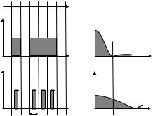
Figure 11.5 shows both variants: The right part depicts the spectrum obtained for the combined signal. In the final analysis, TDM and WDM use the same amount of bandwidth for the transmission of the same amount of data per unit time.
It is common engineering practice to first combine many telephone channels with TDM to the highest frequency, which can still be conveniently worked with. Resulting data rates are not exactly multiples of 64 kbit/s but slightly more due to an overhead from additional bits required for controlling the decoding. Unfortunately, di erent countries started using di erent numbers of telephone channels for TDM (24 in the USA, 30 in Europe), so that on the transmission lines di erent data rates existed. In order to assure smooth international tra c, a standardization became inevitable.
First the USA created a standard called SONET, for synchronous optical network. The fundamental clock rate is 51.48 Mbit/s and is referred to as OC- 1 (as in optical carrier). Integer multiples of this clock rate may be used; in
Figure 11.5: Comparison of time division multiplex (TDM) and wavelength division multiplex (WDM) formats. For TDM several bit streams are interleaved temporally; the resulting bit rate is the sum of the individual bit rates. For WDM each bit stream is coded onto its own carrier. The right half of the figure shows the spectral composition of both formats; for this example we assume amplitude modulation. All told, both formats occupy the same bandwidth in frequency space.

220 |
Chapter 11. Applications in Telecommunications |
particular, OC-3 at three times that rate (155.52 Mbit/s) and OC-12 at 12 × 51.84 Mbit/s = 622.08 Mbit/s are being used.
By international standardization SDH or synchronous digital hierarchy was created. The fundamental rate is 155.52 Mbit/s; data packets according to this standard are referred to as STM-1 (as in synchronous transport module). Note that OC-3 and STM-1 share the same clock rate.
On long distances, OC-48 signals, or STM-16, are now common; they have ca. 2.5 Gbit/s. For intercontinental tra c, many commercial systems use OC192 (STM-64) at ca. 10 GBit/s. OC-768 or STM-256 at ca. 40 Gbit/s is now introduced. To increase the rate by a factor of 4 presents four times more payload at something like two and a half times the hardware cost; on top of that there are space savings in comparison to four OC-192 sets of hardware. However, at 40 Gbit/s, problems arise that were negligible at lower rates: Polarization mode dispersion becomes a massive problem. This is because the relevance of the e ect is determined by the relative propagation time scatter, i.e., the scatter in units of the clock period. Shorter pulses have a proportionally wider spectrum and thus “feel” more of the dispersion. On the other hand, the clock period shrinks inversely with clock rate. The relative propagation time scatter then grows quadratically with clock rate. For OC-768 signals, it is 16 times as large as for OC-192 signals. Polarization mode dispersion is noticed as a random fluctuation of the state of polarization of the received optical signal which translates to level fluctuations. Quite complex compensation has now been introduced, which can assure glitch-free operation. It may be expected, though, that the next step after 40 Gbit/s will not advance by another leap of a factor of 4 as was the rule so far; rather, it seems now that 100 Gbit/s systems will be the next generation. On the other hand, in laboratory experiments, researchers already explore much higher data rates [160].
11.1.6On and O : RZ and NRZ
The physical representation of a bit value – a zero or a one – in an optical format is usually obtained by intensity modulation of a light wave. Again, there are basically two options; the relative advantages and disadvantages have been under discussion for many years.
Discrete-time signals have a certain clock rate which defines the time slots for the individual bits. To assign a binary value, zero or one, to a time slot one may
either turn the intensity o or on during the entire duration of the time slot; or
place a short signal pulse inside the time slot for a one, and no pulse for a zero.
Figure 11.6 these variants are compared. In the first case, the intensity remains the same during the entire time slot or, in the event of several ones or zeroes in a row, for several clock periods. In the second case, the intensity is always zero when one time slot is over and the next begins. Hence the names no return to zero or NRZ for the first case and return to zero or RZ for the second.
There are two relevant practical di erences. When both zeroes and ones are statistically equally probable, the average for NRZ is 1/2, and for RZ close to
11.1. Multiplexing in Time and Frequency: TDM and WDM |
221 |
bit sequence 0 1 0 1 1 1 0
Time
Amplitude
Spectral
 power density
NRZ
no return to zero
Time |
Frequency |
Amplitude
RZ
return to zero
Time |
Frequency |
T |
1/T |
Time Domain |
Power Spectrum |
Figure 11.6: Comparison of coding binary data in the NRZ and RZ formats. For NRZ the pulse occupies the entire time slot of the clock period T , for RZ just a fraction of it. (In principle the pulse might be much shorter than the time slot; for practical considerations, it is not very much shorter. In the figure, it is about one half.) Shorter pulses have wider bandwidth, so RZ occupies more bandwidth.
zero. This plays a role in the construction of receivers where an AC coupling is usually employed to get rid of 1/f noise and drift.
More relevant is the di erence in usage of frequency space: RZ uses more bandwidth because shorter pulses are spectrally broader. Keeping in mind that bandwidth is a nonrenewable resource, this is not economical. On the other hand, an RZ data stream contains a strong Fourier component at the clock frequency, which makes the design of clock regeneration circuits in the receiver easy. In the case of NRZ less bandwidth is occupied, but in the spectrum of an NRZ signal there is a null at the clock frequency. This is easy to see: for each rising slope in the signal there is also a falling slope. Both types of slopes occur equally often. They therefore introduce Fourier components of the same magnitude but opposite phase at the clock frequency which mutually cancel out. The absence of a strong Fourier component at the clock frequency makes its regeneration more di cult. It can be done by first di erentiating the signal to emphasize the temporal positions of the slopes with a narrow spike, then rectifying the result to make all spikes positive-going. This way one obtains a strong spectral component at the clock rate which can easily be filtered out.
11.1.7Noise
Noise is the collective term for all kinds of external influences that can hamper signal transmission. They include man-made, natural, and fundamental perturbations. The term “noise” must be taken in a broad sense here to denote any type of extraneous material imposed on the signal, be it coherent or incoherent, etc.
Man-made noises include emissions from machinery which find their way into the transmission channel. The reader may have experienced a radio crackling when a car with inadequate radio frequency noise suppression drove by. In the

222 |
Chapter 11. Applications in Telecommunications |
case of wavelength division multiplexing the emissions may arise from other channels: This is then referred to as channel crosstalk.
Natural noises may be caused by electric storms (lightning flashes), solar storms, etc.
Fundamental noises include quantum noise. Any signal is quantized because the basic physical constituents are: Electric currents consist of a certain number of electrons flowing per second and this number is subject to fluctuations. Similarly, any detected light power consists of a certain number of photons received per second; this number, too, fluctuates. The fluctuations constitute the quantum noise. Fundamental noise sources also include thermal noise as it occurs in any electronic circuit. At any temperature other than absolute zero, all constituents of matter including electrons undergo a random motion due to their thermal energy; this produces a noise voltage and a noise current in any real impedance.
Thermal noise can be derived directly from Planck’s distribution formula for radiation [173]; this is indicative of its fundamental nature. One needs to consider the spatial and spectral density (power per frequency interval and per volume element) of a one-dimensional perfect emitter (what physicists call a “black body”) at temperature T . Planck’s distribution in one dimension, written as a function of frequency ν (in Hertz),2 is
Iν dν = |
2hν |
dν. |
(11.6) |
|
hν |
||||
|
|
|
e kT − 1
Here c is the speed of light in vacuum as usual and Boltzmann’s constant k = 1.38 × 10⁻²³ J/K converts temperature to energy units. h = 6.6256 · 10−34 Js is Planck’s constant and hν is the energy of an individual photon.
In the “radio engineering limit” the quantum energy is much smaller than the thermal energy: With hν kT we obtain
Iν dν = 2kT dν;
from this one can deduce the thermal noise as described by Johnson and Nyquist [78, 123], with a “white” spectrum
˜ |
(11.7) |
P = 4kTB , |
˜
where P is the product of open circuit voltage and short circuit current which produces noise in a bandwidth B.
Above that frequency at which hν = kT , the Nyquist–Johnson formula is no longer valid. At standard ambient temperature around 300 K this limit is in the far infrared. Therefore, it is perfectly justified that electronics engineers disregard quantum noise entirely and deal with thermal noise. In the visible and near-infrared optical range, however, quantum noise has the upper hand and quantum e ects present very real limits.
In either case one deals with noise which approaches a Gaussian amplitude distribution and a “white” spectrum; the latter means that the noise’s correlation time is shorter than all correlation times of the signal.
2Most textbooks describe Planck’s law for three-dimensional emitters; for the connection with electronic noise we need the one-dimensional case.
11.1. Multiplexing in Time and Frequency: TDM and WDM |
223 |
Fundamental Limitations Due to Noise
In the most favorable case that all technical and thermal sources of noise are negligible, there is quantum noise left and presents a limit to transmission. Let us assume binary coding and estimate the limit of reach. We will keep in mind that in terms of realistic systems the following is far too optimistic; we are after the ultimate limit.
As discussed in Sect. 5.4, there must be at least a single photon received for a signal to be detectable. (We are serious about the ultimate limit!) The photon energy is E = hν ≈ 6.6 ×10−34 Js ×200 ×1012 Hz ≈ 10−19 J in the near infrared. The average launch power is limited to around 1 W so that thermal damage to the fiber is avoided, this corresponds to 1019 photons/s. Then an attenuation of no more than 1/1019 or 190 dB is admissible when we assume for simplicity the ridiculous bit rate of 1 bit/s. We also accept that due to the statistical nature of the photon number in some cases, zero photons will be detected instead of one; this would constitute a transmission error, and we will come to that. For a fiber with 0.2 dB/km, this gives a maximum distance of 950 km.
Due to energy loss, optical fibers are quantum limited in their reach. Even in an unrealistically optimistic estimate the maximum distance is less than 1000 km.
Distances spanned in practical systems are much shorter than that; hence the requirement of optical amplifiers.
Of course it is not possible to detect a signal consisting of a single photon without error, due to the statistical nature of both their generation and their detection. Therefore it is useful refine our estimate as follows: We set an upper limit to the bit error probability which is deemed su cient for practical purposes, and calculate how many photons on average must be contained in a light pulse to accommodate that limit. For the distribution of photon numbers we may assume Poisson statistics. At an average photon number N , the probability to have the value n (do not confuse this symbol with the refractive index!) is
given by
p(n) = N n e−N /n!.
Then, the probability to erroneously measure a logical “one” when indeed a
“zero” was sent is
p(1) = 01 e−0/1! = 0.
Zeroes are detected error-free! This is no surprise because when zero photons are sent, and all other noise sources are excluded, the arriving number of photons got to be zero. For the “ones” it is di erent: The probability to measure a “zero” when in fact a “one” was sent is
p(0) = N 0 e−N /0! = e−N .
In the telecommunications industry it is common to set the maximum allowed bit error rate in telephony to 10−9. We insert this value and solve for N . On average, there are as many “zeroes” as there are “ones”, but “zeroes” are detected error-free. Then we can admit an error of 2 × 10⁻⁹ for the “ones”. It
follows that
Nmin = ln 2 × 10−9 = 20.03.
In an ideal situation it would su ce to have 20 photons for a “one”:
224 |
Chapter 11. Applications in Telecommunications |
In order to detect a signal with a bit error rate below 10−9, photon statistics dictates that a logical symbol on average must contain at least 10 photons.
In any practical context other sources of noise and error will also contribute; therefore even the best available detectors require at least ten times as many photons, and typical decent detectors maybe a hundred times as many. Detectors that are uncompromisingly optimized for highest speed may require even more than that.
11.1.8Transmission and Channel Capacity
Now we consider the compound signal coded in one of the formats described above: RZ or NRZ; TDM and/or WDM. This signal is eventually fed to a receiver. The idea is that this occurs across a certain distance; this implies that over the distance there is some suitable transmission medium, like a cable. The medium acts as a channel.
External noises and perturbations also act on the channel; as a result, what arrives at the receiver is a mix of the signal proper and some noise. It is the task of the receiver to reconstruct the signal without error and to disregard the noise. That may or may not be possible. This is the topic of communications theory, a field which was started by a seminal work by Claude Shannon [137].
Shannon’s work shows that one of the most relevant parameters is the bandwidth available for the transmission. Assuming that the channel can provide the bandwidth B, transmission can take place with a data rate R as long as R remains smaller than the channel capacity C. The latter is defined by
C = B |
· |
log |
|
1 + |
|
S |
. |
(11.8) |
2 |
|
|
||||||
|
|
|
N |
|
||||
Here S is the signal power and N the noise power. Noise is assumed to be Gaussian white noise. Shannon showed that provided R < C, a coding can be found such that the bit error rate can be made arbitrarily small. It is well possible that the coding gets increasingly complex as R approaches C (from below), but virtually error-free transmission is possible. If, on the other hand, transmission with R > C is attempted, the bit error rate can no longer be kept down.
According to Eq. (11.8), the dominant factor determining the channel capacity is the bandwidth. One might think, then, that an infinite amount of data can be transmitted when B is allowed to grow indefinitely. This is not so. The catch is that the noise also depends on bandwidth. If one restricts the discussion to white noise, the noise power is proportional to bandwidth. Then one can write N = N0B, with N0 = const. the spectral noise power density which is constant. In the limit
Blim C = ∞, |
||||
→∞ |
|
|
|
|
it follows that |
S |
|
||
Blim C = |
· log2 e. |
|||
|
|
|||
N |
|
|||
→∞ |
|
0 |
|
|
In reality, of course, the available bandwidth cannot grow indefinitely anyway but is bounded by physical considerations.
11.2. Nonlinear Transmission |
225 |
Transmission through optical fiber, in comparison to electric cables, enjoys the benefit of a wide spectral region of low loss. If we take the regime of the third window generously as 1,400–1,600 nm corresponding to a frequency interval of 214–188 THz, the bandwidth is 26 THz. With the best available fibers, one may be able to utilize an even more extended range of (optimistically) 1,250– 1,650 nm; this corresponds to 240–180 THz implying a bandwidth of 60 THz. Of course, toward the end points of this interval, losses are much higher than in the middle so that for long-distance transmission one may be tempted to return to a less optimistic estimate. In any event, realistic estimates produce bandwidths on the order of 50 THz.
The spectral e ciency
η = |
R |
Bits/s/Hz |
(11.9) |
|
B |
||||
|
|
|
indicates how well the data rate makes use of the available bandwidth. For binary signals only two values are used: o and on, or zero and some power at least equal to noise power. This can be formally introduced into Eq. (11.8) by letting S = N ; then we obtain
C = B |
channel capacity for binary transmission. |
(11.10) |
In other words, for binary transmission the maximum rate is 1 bit/s in 1 Hz of bandwidth.
11.2Nonlinear Transmission
In long-haul transmission, it is unavoidable that the fiber’s nonlinearity becomes noticeable. Nonlinearity is special because in electrical cables both attenuation and dispersion are well known, but a phenomenon corresponding to the Kerr nonlinearity in fiber does not exist. This may be why engineers trained in electronics instinctively considered nonlinearity as an impediment and an utter nuisance for a long time. The way to avoid nonlinearity, in this logic, is to use large-mode area fibers to reduce the nonlinear coe cient and to use low power signals. This approach can go a long way. Indeed, in a remarkable experiment, a data transmission rate of 1 Tbit/s over 300 km has been demonstrated [160]. Only a few researchers pointed out as early as in the 1980s that nonlinearity also presents an opportunity to counteract dispersion’s detrimental e ects and thus to improve the transmission system as a whole. Both approaches are being pursued, and only the future can tell which one will ultimately be better.
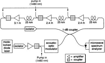
Before any commercial system can be deployed, there are years of extensive research experiments and laboratory tests, and finally field trials. Lab tests are not done in actual long-distance optical cables but in closed fiber loops which can be set up in a laboratory. Signal degradation with distance can then be assessed in detail by just letting the signal go around the loop for more and more turns; Fig. 11.7 shows what insiders tongue-in-cheek call a carousel.
Much research deals with that paradigm of transmission in the presence of Kerr nonlinearity, the fundamental (i.e., N = 1) optical soliton. Solitons are the natural units (bits) for transmission of data over optical fibers because they are more robust than any other type of pulse. They require anomalous fiber
226 |
Chapter 11. Applications in Telecommunications |
Figure 11.7: A typical laboratory experiment for the study of long-distance transmission. The long distance is here represented by multiple round trips in a fiber ring. In this example, the ring has 75 km circumference and contains three amplifiers. From [114] with kind permission.
dispersion; it comes in handy that the spectral regime of lowest loss coincides with the anomalous dispersion regime.
According to the latest research, the best results are obtained not with pure solitons but rather with a certain generalization of the soliton concept. A number of subtle e ects become noticeable on truly long distances on the order of thousands of kilometers, some in an individual wavelength channel and others only in the case of WDM. These e ects make the situation a little more complex; it is then a matter of taste whether one still calls the modified pulses by the name of solitons or by some other name. A few books have recently become available that are devoted to solitons in optical fiber [61, 17, 115].
11.2.1A Single Wavelength Channel
In spite of their extraordinary stability, solitons do not enjoy eternal life. Perturbations arise from energy loss, Raman scattering, and by mutual interactions of pulses (see above). Combined, they eventually destroy even solitons [99, 31].
Energy loss may be compensated by optical amplifiers (of the Raman type or with Er-doped fiber) at least on average. The first question to ask is at which intervals Lamp one should insert amplifiers into the fiber. It turns out that the condition LD Lamp must be maintained in order to avoid a resonant perturbation of the solitons [59, 60, 26, 115]. For typical standard fiber and picosecond pulses, LD is a few to a few tens of kilometers. Here is a quick estimate:
|
T 2 |
|
(10 ps)2 |
||
LD = |
0 |
= |
|
|
= 5 km. |
|β2| |
20 ps2 |
|
|||
|
|
/km |
|||
It would be awkward to insert amplifiers at distances shorter than this. If dispersion is reduced to 1 ps/(nm km), however, and if pulse durations are in the single-digit picosecond range, LD becomes a few hundred kilometers. Then, very reasonable intervals between amplifiers on the order of tens of kilometers
11.2. Nonlinear Transmission |
227 |
are possible. A useful side e ect of low-dispersion fiber is that the soliton’s energy is also scaled down so that less power is required for their generation. Also, the combined power of possibly a hundred WDM channels is kept low so that handling live fibers does not pose a health hazard to a service crew. On the other hand, one should not push dispersion reduction too far because there is also a signal-to-noise issue when the soliton energy goes down too much.
Gordon–Haus E ect
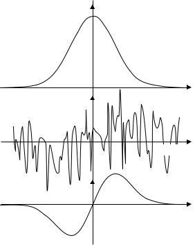
Amplifiers, by their nature, cause additional noise due to spontaneous emission; this noise degrades signal integrity in a subtle manner. It modifies the pulse energy, its optical phase, and its temporal position. Modifications of amplitude, phase, and position of solitons are not a big worry. However, frequency deviations spell trouble. They arise from asymmetric components of the noise with respect to the spectral center of the pulse (see Fig. 11.8). In the presence of dispersion, frequency changes produce changes in the pulse arrival time, which, after a long distance, add up to a considerable random pulse jitter. If the jitter becomes too large (i.e., comparable to the clock period), the signal is rendered unreadable. This phenomenon is called Gordon–Haus jitter [55] in honor of James P. Gordon and Hermann A. Haus who predicted it. They showed that the jitter grows with the third power of distance.
signal pulse
Frequency
noise
Frequency
Frequency
noise component
Figure 11.8: With respect to the pulse spectrum (top), noise (center ) may have asymmetric components (bottom). If noise is then added to the pulse, the spectral center-of-mass (i.e., the center frequency) is shifted ever so slightly. Due to dispersion in the fiber, this results in a modified time of arrival. These random fluctuations of arrival time are called Gordon–Haus jitter.
228 |
Chapter 11. Applications in Telecommunications |
Time (ps)
60
40
20
0
0
eff. pulse duration
Gordon-Haus limit
scatter
2 |
4 |
6 |
8 |
10 |
Distance (Mm)
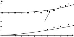
Figure 11.9: Experimental demonstration of Gordon–Haus jitter. The apparent increase of pulse width with increasing distance is in perfect agreement with the prediction. From [112] with kind permission.
The existence of the Gordon–Haus jitter was clearly shown experimentally (Fig. 11.9). In the experiment, it was necessary to average over many consecutive pulses so that the arrival time jitter appeared like a pulse broadening. The apparent increase of pulse width with distance followed precisely the prediction of the jitter [112].
Filters Along the Line
Insight about Gordon–Haus jitter was the reason why in the transatlantic cables TAT-12 and TAT-13 (see below) dispersion shifted fiber and Er-doped fiber amplifier were used, but solitons were not. However, only a short time later a remedy was found: Wavelength-selective filters reduce frequency fluctuations as they continuously nudge solitons back to the center of their spectral slot. Moreover, in a wavelength division multiplexed (WDM) system, di erences in gain from one wavelength channel to the next are equalized by filters because if one pulse is momentarily too powerful, it acquires a broader spectrum through self-phase modulation; at the next filter, it then su ers greater loss which brings its power back to normal [113]. This is shown in Fig. 11.10.
Of course the scheme mandates that filters are placed at certain intervals along the line; for practical, reasons one chooses the same positions as the amplifiers. On a transoceanic distance there will then be many filters cascaded. It is well known that for cascaded elements in a linear system, the resulting frequency response is the product of the individual filter responses. That statement here implies that a very narrow spectral transmission results. Within this narrow width spontaneous emission can still grow unhindered and will pose a problem.
Again a very simple idea presents an elegant solution to this problem. All filters do not have the same center frequency; rather, the center frequencies are sliding along the line. Then there is no single wavelength for which spontaneous emission can transit the whole distance because in the product of filter responses, there is always one factor practically zero for any frequency. For linear signals, a sliding filter system is opaque! For solitons it is di erent: Solitons are creatures of the nonlinear realm. They can adjust their shape and center frequency at each filter and thus pass through the entire system without any problem. Such a discrimination between signal and noise has no correspondence in linear systems!