

Fiber_Optics_Physics_Technology
.pdf9.4. Solutions of the NLSE |
177 |
Distance |
Power |
Time |
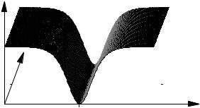
Figure 9.17: An N = 4 soliton in a computer simulation, shown from 0 to 2z0.
Distance |
Spectral |
power |
Frequency |
Figure 9.18: Spectrum of an N = 4 soliton in a computer simulation, in correspondence with Fig. 9.17.
(Fig. 9.19). From the tanh function, they inherit the special property that a phase jump of π occurs at center.
Both in experiment and numerical simulation, one does not have the chance to work with an infinitely wide bright background. A good approximation can be found by using a background pulse of considerably longer duration. Of course, this background pulse, by way of its large width, contains much more energy than a comparable bright soliton; this seems to make dark solitons not very attractive for optical data transmission. On the other hand, they are less sensitive to a variety of perturbations than bright solitons, and some authors pursue them as an alternative. In practical terms, in reported experiments on dark solitons, it was already di cult to produce them in the first place.
Strictly speaking, the dark solitons just described are called black solitons. The reason is that black solitons are only one member of a wider class of dark solitons which di er in the depth of the intensity minimum. There are dark pulses which do not dip down all the way to zero and which are called gray solitons. The general solution of the nonlinear Schr¨odinger equation for dark solitons is
|
1 |
|
|
i ϕ(τ )+( |
A0 |
)2ξ |
|
|
|
B |
|||||
u(ξ, τ ) = A0 |
|
− sech(A0τ ) e |
(9.56) |
||||
B2 |
|||||||
178 |
Chapter 9. Basics of Nonlinearity |
Power
Distance
Time
Figure 9.19: A dark soliton in a computer simulation. In comparison to Fig. 9.5, here all parameters are the same with the exception of the sign of dispersion; β2 = −18 ps2/km has been changed to β2 = +18 ps2/km.
with the abbreviations |
|
|
|
|
|
|
|
|
|
|
|
|
|
|
|
A02 |
|
|
|
|
|
||||
τ = A0 |
τ + |
|
1 |
− |
B2 |
ξ |
||||||
|
|
|||||||||||
|
|
|
B |
|
|
|
|
|
|
|||
and |
|
|
|
|
B tanh(t) |
|
|
|||||
ϕ(t) = arcsin |
|
|
|
|
. |
|||||||
|
|
|
||||||||||
|
|
|||||||||||
|
1 |
− B2sech2(t) |
||||||||||
The amplitude factor A0 fixes the brightness of the background and B defines the “grayness”. In the limit limB→1 gray turns black, in a manner of speaking, and Eq. (9.56) reproduces the solution A0 tanh(A0τ ). In this case there is the abrupt phase jump of π at soliton center; for gray solitons, the phase transits in a continuous way, not stepwise.
9.5Digression: Solitons in Other Fields of Physics
Solitons, that is, nonlinear waves with special properties, certainly do not exist solely in optical fibers. Indeed, the term was coined following observations in other branches of science. The first reported conscious observation of a soliton phenomenon was written by a Scotsman, the civil engineer John Scott Russell. In 1838 he noticed a remarkable water wave in the Union Canal near Edinburgh and wrote this report [132]:
I was observing the motion of a boat which was rapidly drawn along a narrow channel by a pair of horses, when the boat suddenly stopped – not so the mass of water in the channel which it had put in motion; it accumulated round the prow of the vessel in a state of violent agitation, then suddenly leaving it behind rolled forward with great velocity, assuming the form of a large solitary elevation, a rounded, smooth and well-defined heap of water, which continued its course along the channel apparently without change of
9.5. Digression: Solitons in Other Fields of Physics |
179 |
form or diminution of speed. I followed it on horseback, and overtook it still rolling on at a rate of some eight or nine miles an hour, preserving its original figure some thirty feet long and a foot and a half in height. Its height gradually diminished, and after a chase of one or two miles I lost it in the windings of the channel.
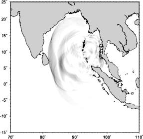
A first attempt at a mathematical explanation was not published until 1895 when Diederik Korteweg and Gustav de Vries formulated a hydrodynamic wave equation. It was only after their work that in the interplay of dispersion and nonlinearity solitary waves became an expected feature. Their hydrodynamic wave equation is now called the Korteweg-de-Vries equation (KdV equation). It di ers from the nonlinear Schr¨odinger equation of fiber solitons, which concerns us here, and therefore its solutions are somewhat di erent, too. One important di erence is that unlike in the nonlinear Schr¨odinger equation, in the KdV equation the speed of propagation becomes amplitude-dependent. This is why water waves move faster in deep water than in shallow water, a fact which has considerable, indeed dramatic consequences in the case of a tsunami (Japanese for harbor wave). Triggered by undersea earthquakes, water surface waves with enormous energy propagate at rapid speed across the ocean, but they do so with extremely long wavelength and low amplitude. They therefore easily go unnoticed, but they can cross all of the Pacific Ocean within 2 days. As they approach a shore where the water depth is reduced, the energy transport remains conserved, but since the speed is reduced, the amplitude must increase and may generate crests of 20 m elevation. If such a wave hits a shore it will destroy whatever gets in its path. In December 2004, this happened in a particularly sad form when a quake o Sumatra triggered an Indian Ocean tsunami which wreaked havoc in Indonesia, Thailand, Sri Lanka and on to the East African shores and took about a quarter million human lives (Fig. 9.20).
Figure 9.20: A model calculation for the Indian Ocean tsunami on December 26, 2004. This is one frame of an animation, taken from [74] with kind permission.

180 |
Chapter 9. Basics of Nonlinearity |
In 1965, Norman Zabusky and Martin Kruskal studied interactions of solitary waves [165] and noticed their particle-like properties. Solitons can be reflected o each other without any harm to their structure. The moniker “soliton” reminds us of elementary particles.
Application of the soliton concept to fiber optics started in 1971 when Vladimir Evgen’evich Zakharov and Alexey B. Shabat [166] formulated a wave equation for pulse propagation in fibers and found solitonic solutions. In 1973, Akira Hasegawa and Frederick Tappert predicted [62] that such optical solitons should be observable experimentally and that they hold promise for optical data transmission. Linn F. Mollenauer and collaborators succeeded in 1980 to experimentally demonstrate the existence of fiber solitons [111]. Then, various aspects of optical solitons were subject to closer investigation. F. Mitschke and Mollenauer showed the particle properties in 1986 by demonstrating for the first time the interaction forces between fiber-optic solitons [106].
In a slightly di erent context also in optics, spatial or transverse solitons in various media are studied. These are beams of light which stabilize their crosssectional shape in the presence of nonlinearity and di raction, in very close analogy (if one accepts to switch the roles of time and space) to the solitons described here. However, spatial solitons do not occur in fibers and are therefore beyond the scope of this book. The reader interested in a comparison is referred to [19, 167, 128, 85].
9.6More χ(3) Processes
In our approach to derive a wave equation, we have assumed a monochromatic wave. Then we found self-phase modulation, an e ect by which a monochromatic wave or, in extension, a more or less narrowband light pulse modifies itself. But this is not the only consequence arising from third-order susceptibility χ(3). It also gives rise to the following e ects:
Cross-phase modulation. In the presence of an intensive wave of frequency ω, a wave of frequency ω + ω gets phase modulated.
Frequency tripling. A new wave of frequency 3ω arises from a wave of frequency ω.
Four-wave mixing. The three fields involved in a χ(3) process may, in the most general case, all have di erent frequencies. Then, new frequency components arise at combination frequencies.
Cross-phase modulation arises because the index modulation created by one wave also has an influence on the other wave. Frequency tripling, also known as third harmonic generation, can be understood in either one of two ways: In the wave picture, the light field acting on an atom can be written as an oscillation of the type sin ωt. In a χ(3) process, there are three waves acting simultaneously. All three may have the same frequency: Then there is a term sin3(ωt) = 14 (3 sin ωt − sin 3ωt) containing the third harmonic. In a particle picture, there are three photons acting on the atom simultaneously. It absorbs three times the energy of a single photon. The probability of this process rises with the third power of the photon density because it takes three simultaneously arriving photons. Also, the process becomes much more probable when an atomic energy level exists at or near E = 3 ω.
9.6. More χ(3) Processes |
181 |
In the same way, one can discuss four-wave mixing: In the wave picture the three irradiated waves may all have di erent frequencies. Then, one can use a relation between trigonometric functions of the type
sin ω1t · sin ω2t · sin ω3t = |
|
|||
1 |
|
sin(ω1 + ω2 + ω3)t + sin(−ω1 + ω2 + ω3)t |
|
|
|
4 |
|
|
|
+ |
sin(ω1 − ω2 + ω3)t + sin(ω1 + ω2 − ω3)t . |
(9.57) |
||
There are four combination frequencies, hence the name of the process. In the particle picture, there are three photons acting on an atomic medium. Both absorption or stimulated emission can occur. If all three photons are absorbed, the atom stores an energy equal to the sum and can reradiate a wave with the corresponding frequency. The other combination tones occur when one of the photons stimulates an emission. (The loss of energy from the atom is reflected in the negative sign in the respective term of Eq. 9.57.)
For our purposes, the following remark is important: In the special case that all ωi are integer multiples of a certain fundamental frequency ω0, then the same is also true for all combination frequencies: Let k, l, m N. Then, if ω1 = kω0, ω2 = lω0, and ω3 = mω0, it follows that the combination frequencies are (k + l + m)ω0, (−k + l + m)ω0, (k − l + m)ω0, and (k + l − m)ω0, all integer multiples of ω0. In the special case called degenerate four-wave mixing, two
of the three frequencies are the same. Let, e.g., ω1 = ω2 |
and ω3 = ω1 + |
ω. |
Then the fourth wave has the frequency ω4 = ω1 − ω. |
As a result, a pair |
|
of frequencies separated by ω will produce two new frequencies. One is |
ω |
|
below the lower frequency, and the other ω above the higher frequency. |
|
|
This consideration is simplified insofar as it makes no statements about the intensities of the generated waves. In order to assess that aspect we need to consider the following.
Let us assume that energy is transferred through some nonlinear mixing process from one wave to another. Both propagate through the material in the same direction. In general their frequencies will di er, and in the presence of dispersion they have di erent phase velocities. This implies that their relative phase will wander as they propagate.
As is well known from coupled oscillators, energy always flows from that with advanced phase to that with retarded phase. The energy transfer is most e cient if the phase of the driving oscillator is 90◦ advanced with respect to the driven oscillator. This can be generalized to traveling waves.
Right after the launch point, energy from wave A feeds wave B which at this point just emerges. The phase of wave B is automatically arranged such that an energy transfer takes place. A certain distance down the fiber, both waves have experienced a relative phase shift of 90◦ and energy transfer ceases. A little further on, the phase of wave B is advanced and energy is transferred back!
Instead of an unlimited increase of the energy of wave B, there is a periodic exchange of energy between both waves. This becomes noticeable at the point where the relative phase is rotated by 90◦ for the first time. If a most e ective energy transfer is desired, one has to make this distance long; the most obvious means to do that is to make dispersion small. The technical term is phase matching of both waves. If, on the contrary, one wishes to thwart the energy

182 |
Chapter 9. Basics of Nonlinearity |
transfer, one can arrange for strong dispersion. We will look closer into this logic in Sect. 11.2.3.
9.7Inelastic Scattering Processes
An important class of nonlinear processes in fibers are scattering processes in which light is scattered by the medium (glass) either elastically or inelastically. In the case of elastic scattering, the energy of the light quanta, and thus the frequency, is unaltered. This puts elastic scattering into the realm of linear optics. We have already discussed Rayleigh scattering, a process in which scattering occurs in all directions, creating a linear loss: a loss of photons in proportion to the existing number of photons.
For inelastic scattering processes, an amount of energy δE is exchanged with the medium (either absorbed by the medium or released). Since δE = hδν, there is a frequency shift δν. Two types of inelastic scattering processes in fibers are distinguished: Brillouin scattering and Raman scattering. These are scattering processes either at the acoustic (Brillouin) or optical (Raman) phonon branch. In either case, in principle there can be an upshift or downshift of frequency. The irradiated wave is called pump wave; the scattered wave is called the Stokes wave in case of downshift, and the anti-Stokes wave in the case of upshift.
Almost always the downshift (Stokes wave) is much more pronounced. The medium usually consists of atoms or molecules which are in or near their energetic ground states, as given by the thermal energy and a Boltzmann distribution of occupation numbers. Then the medium can absorb, but not release energy.
Photons can be scattered spontaneously in both cases, but the rate is low. On the other hand, beginning at a certain threshold intensity a stimulated scattering process sets on. This is then called stimulated Raman scattering (SRS), or stimulated Brillouin scattering (SBS). The process can become stimulated when a su cient number of spontaneously generated photons is already present and interacts with the pump wave. Then the polarization of the medium is driven, and above the threshold the process grows exponentially. Of course this exponential growth of Stokes or anti-Stokes wave cannot go on indefinitely: eventually the pump is depleted so that further growth is halted.
To get an idea of all this in more quantitative terms, we use the following rate equation model: Let Ns be the number of Stokes photons and Np the number of pump photons. Then, in the stimulated process, we have
dNdzs = const. Np(Ns + 1).
The “1” inside the parenthesis is for the spontaneous rate without which the process can never start (just like in a laser). Once the startup phase is over, the spontaneous rate may be neglected in comparison to Ns. Then there is a solution
Ns(z) = Ns(0) exp(gIz),
where g is the gain coe cient for the Stokes wave.
By exponential growth even a single spontaneously occurring photon may produce a macroscopic light wave. Macroscopic means that the growth continues until the energy of the pump wave is noticeably depleted. Then a limit to growth is reached – but this does not necessarily imply a steady equilibrium. Quite to the contrary, it has been shown for Brillouin scattering in fibers that the Stokes
9.7. Inelastic Scattering Processes |
183 |
wave has strong, irregular power fluctuations which can be interpreted as the remainder of the stochastic signature of the startup process.
The stimulated scattering process can have profound impact on a light wave propagating in a fiber. Often this is a detriment, which can in no way be neglected. On the other hand, we will see that the influence is not always unwelcome, but can also be harnessed to perform useful functions.
It goes without saying that in any scattering process, conversation of both energy and momentum must hold. We can write that as
ω = |
ω, |
(9.58) |
in |
out |
|
k = |
k. |
(9.59) |
in |
out |
|
On the LHS, there are all waves entering the interaction process, and on the RHS all waves that exit from the process.
9.7.1Stimulated Brillouin Scattering
We begin by considering the case of Brillouin scattering in which an acoustic wave is generated.
ωp |
= |
ωs + ωa, |
(9.60) |
kp |
= |
ks + ka. |
(9.61) |
Indices p, s, and a refer to pump, Stokes, and acoustic waves, respectively. Pump and Stokes waves oscillate at optical frequencies while the acoustic
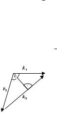
wave has a considerably lower frequency. Therefore the wave vectors for pump and Stokes wave will be similar and much larger than that of the acoustic wave. We can therefore approximate that |kp| ≈ |ks| and ωa ωp, ωs. Referring to Fig. 9.21, we can then write
θ
|ka| = 2|kp|sin 2
with θ the angle between the propagation directions of pump and Stokes waves. The pump wave propagates along the fiber, and so θ is also the angle with the fiber axis for the Stokes wave.
A wave vector equals angular frequency divided by velocity, so that
θ
ωa = va|ka| = va2|kp|sin 2 .
Figure 9.21: Sketch for the relation between three wave vectors involved in Brillouin scattering and the angle θ. This is very nearly an equilateral isosceles triangle, and therefore the perpendicular halves both |ka| and θ. Then |ka|/2 = |kp|sin(θ/2).
184 Chapter 9. Basics of Nonlinearity
va is the velocity of sound, which in fiber is 5960 m/s.
We see that the Stokes shift ωa depends on θ and disappears in forward direction (θ = 0). This gives rise to conflict with energy conservation except when the energy of the forward-scattered wave vanishes. In backward direction, on the other hand, the frequency shift acquires its maximum. The physical interpretation can be given as a Doppler e ect of a wave which is scattered o a grating traveling itself with the velocity of sound. Directions other than forward and backward are not relevant in fibers, and single-mode fibers in particular. (Strictly speaking, SBS does not entirely vanish in forward direction; there is a minimal forward scattering known as GAWBS (guided acoustic wave Brillouin scattering), which is several orders of magnitude weaker than backward scattering.)
Signal(arbitraryunits) |
|
|
|
|
|
10.6 |
10.8 |
11.0 |
11.2 |
11.4 |
|
Frequency (GHz)
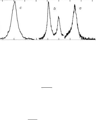
Figure 9.22: Brillouin scattering spectrum for three di erent fibers. (a) undoped silica core, (b) depressed-clad fiber, (c) dispersion shifted fiber. In all cases the shift is near 10 GHz. From [155] with permission.
If we rewrite in terms of natural, rather than angular frequencies and use index “B” for “Brillouin”, the Brillouin shift is given by
νB = |
ωa |
= |
2va|kp| |
= 2va |
n |
|
2π |
2π |
λp |
||||
|
|
|
because |kp| = 2πn/λp. If for example n = 1.46 and λp = 1.55 μm, one obtains νB = 11.2 GHz. As a general statement, SBS produces frequency shifts on the order of 10 GHz, which is a relative shift of 10−4 (Fig. 9.22).
The change of Stokes power with distance along the fiber can be described
by
dIs |
= gIpIs − αsIs. |
(9.62) |
d(−z) |
Indices refer to Stokes and pump wave as before. The derivative here has been taken with respect to (−z) because for SBS the scattered wave travels backward. The frequency of the acoustic wave is so much smaller than the optical frequencies that we may write ωp/ωs ≈ 1 and αs ≈ αp. The gain factor g for SBS is about gB = 20 pm/W, slightly lower than for bulk fused silica with about gB ≈ 50 pm/W.
The corresponding equation for the pump wave reads |
|
||||
|
dIp |
= − |
ωp |
(9.63) |
|
|
|
|
gIpIs − αpIp. |
||
|
dz |
ωs |
|||
9.7. Inelastic Scattering Processes |
185 |
It is easy to check that for the lossless case (αs = αp = 0), the following holds:
d |
|
Is |
− |
Ip |
= 0. |
dz |
ωs |
ωp |
|||
This demonstrates the conservation of photon number.
The first term on the RHS of Eq. (9.62) is the gain, the second, loss. Correspondingly, in Eq. (9.63) the first term is for saturation, the second, loss. We now ask for the threshold pump power for the generation of the stimulated effect. Surely, close to that threshold, the Stokes wave is still weak so that we can neglect saturation to obtain an expression for the threshold:
|
dIp |
= |
−αpIp, |
|
|
|||||
|
|
dz |
|
|
||||||
|
Ip(z) = Ip0e−αpz , |
|
||||||||
|
dIs |
= gIsIp0e−αpz − αsIs |
||||||||
|
d( z) |
|
||||||||
|
− |
= Is gIp0e−αpz − αs . |
||||||||
|
|
|
|
|||||||
As we integrate, the first term in parentheses yields |
||||||||||
L Ip0e−αpz dz = |
|
Ip0 |
1 |
− |
e−αpL |
= Ip0Le . |
||||
|
||||||||||
0 |
|
|
|
|
|
αp |
|
|
||
Now we solve
Is(0) = IsL exp (gIp0Le − αsL) .
By convention, a useful criterion for threshold is that (in the absence of saturation) Is,max = Ip,min. As initial value for the Stokes wave, one assumes a single photon inserted at the (near or far, whichever applies) fiber end to generate spontaneous scattering. Figure 9.23 clarifies to which positions the quantities are referred.
As for values of the gain coe cient, strictly speaking they depend somewhat on spectral line shape, the state of polarization of both waves, etc. However, as a reasonable order of magnitude, we may use gIp0Le ≈ 20. If one inserts the
above values of g and Le ,max, one finds a threshold of 2.5 mW in a fiber with Ae = 50 μm2.
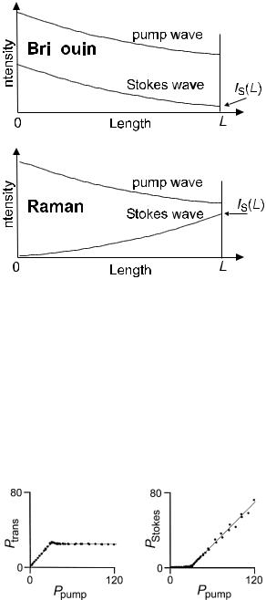
This extremely low value renders stimulated Brillouin scattering the nonlinear process with the lowest threshold. SBS gets in the way whenever continuous wave experiments are considered. One important consequence is a severe limitation of the fiber’s ability to transmit power: As soon as the pump wave exceeds threshold, the excess is transferred into a Stokes wave which travels back to the light source. Figure 9.24 shows an experimental result to illustrate this point. Continuous wave light with adjustable power from a dye laser is launched into a single-mode fiber. At the distal fiber end, after about 100 m fiber length, a detector monitors the transmitted power. Power scattered back inside the fiber is diverted with a beam splitter at the near fiber end and is fed to a second detector. It is quite obvious that the linear relation between launched and transmitted power ends at some point, in this example at about 20 mW. Whatever power in excess of this threshold is launched is scattered back and appears at the other detector.
186 |
|
|
|
Chapter 9. Basics of Nonlinearity |
|
|
|
|
|
|
|
|
|
|
|
|
|
|
|
|
|
|
|
|
Figure 9.23: Sketch to explain the spatial evolution of pump wave and Stokes wave in stimulated Raman and Brillouin scattering.
The threshold can be lowered even further when power traveling in the fiber is recycled by reflection at the fiber ends. The main e ect is that by back reflection, a coherent wave can seed the Stokes wave; this is more e cient than a spontaneous photon. It has been shown that the minute natural Fresnel reflection at the fiber ends has appreciable influence.
The temporal structure of the backscattered wave is not at all continuous. The Stokes wave is deeply and irregularly modulated (see Figs. 9.25 and 9.26). This is a signature of the stochastic nature of spontaneous scattering. In the
Figure 9.24: Experimental observation of stimulated Brillouin scattering in a fiber. All powers are given in milliwatt. Left : Above threshold of stimulated Brillouin scattering the power of a continuous wave laser that is transmitted through the fiber is clamped. Right : The power “missing” in transmission appears in the backscattered Stokes wave.