in some detail by Arzeliès (1966), Marder (1971), and Terletskii (1968). For a scientific biography of Einstein, see Pais (1982).

Our interest in SR in this text is primarily because it is a simple special case of GR in which it is possible to develop the mathematics we shall later need. But SR is itself the underpinning of all the other fundamental theories of physics, such as electromagnetism and quantum theory, and as such it rewards much more study than we shall give it. See the classic discussions in Synge (1965), Schrödinger (1950), and Møller (1972), and more modern treatments in Rindler (1991), Schwarz and Schwarz (2004), and Woodhouse (2003).

The original papers on SR may be found in Kilmister (1970).

1.13 A p p e n d i x : T h e t w i n ‘ p a ra d ox ’ d i s s e c t e d

The problem

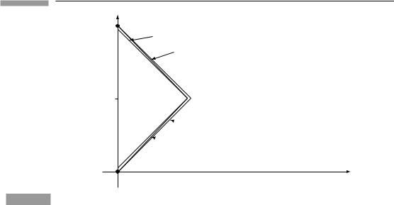
Diana leaves her twin Artemis behind on Earth and travels in her rocket for 2.2 × 108 s (≈ 7 yr) of her time at 24/25 = 0.96 the speed of light. She then instantaneously reverses her direction (fearlessly braving those gs) and returns to Earth in the same manner. Who is older at the reunion of the twins? A spacetime diagram can be very helpful.

Brief solution

Refer to Fig. 1.16 on the next page. Diana travels out on line PB. In her frame, Artemis’ event A is simultaneous with event B, so Artemis is indeed ageing slowly. But, as soon as Diana turns around, she changes inertial reference frames: now she regards B as simultaneous with Artemis’ event C! Effectively, Diana sees Artemis age incredibly quickly for a moment. This one spurt more than makes up for the slowness Diana observed all along. Numerically, Artemis ages 50 years for Diana’s 14.

Ful ler discussion

For readers who are unsatisfied with the statement ‘Diana sees Artemis age incredibly quickly for a moment’, or who wonder what physics lies underneath such a statement, we will discuss this in more detail, bearing in mind that the statement ‘Diana sees’ really means ‘Diana observes’, using the rods, clocks, and data bank that every good relativistic observer has.

Diana might make her measurements in the following way. Blasting off from Earth, she leaps on to an inertial frame called O¯ rushing away from the Earth at v = 0.96. As soon as she gets settled in this new frame, she orders all clocks synchronized with hers, which read ¯t = 0 upon leaving Earth. She further places a graduate student on every one of her

Diana’s change of frame is analogous to a rotation of coordinates in Euclidean geometry.

Figure 1.17

does it matter, after all, that they would have sent her dispatches dated ¯t = 171 yr? Time is only a coordinate. We must be sure to catch all the events.

What Diana really did was use a bad coordinate system. By demanding information

only before ¯t = 7 yr in the outgoing frame and only after = 7 yr in the ingoing frame, t

she left the whole interior of the triangle ABC out of her coordinate patches (Fig. 1.17(a)). Small wonder that a lot happened that she did not discover! Had she allowed the first frame’s students to gather data until ¯t = 171 yr, she could have covered the interior of that triangle.

We can devise an analogy with rotations in the plane (Fig. 1.17(b)). Consider trying to measure the length of the curve ABCD, but being forced to rotate coordinates in the middle of the measurement, say after you have measured from A to B in the x − y system. If you then rotate to x¯ − y¯, you must resume the measuring at B again, which might be at a coordinate y¯ = −5, whereas originally B had coordinate y = 2. If you were to measure the curve’s length starting at whatever point had y¯ = 2 (same y¯ as the y value you ended at in the other frame), you would begin at C and get much too short a length for the curve.

Now, nobody would make that error in measurements in a plane. But lots of people would if they were confronted by the twin paradox. This comes from our refusal to see time as simply a coordinate. We are used to thinking of a universal time, the same everywhere to everyone regardless of their motion. But it is not the same to everyone, and we must treat it as a coordinate, and make sure that our coordinates cover all of spacetime.

Coordinates that do not cover all of spacetime have caused a lot of problems in GR. When we study gravitational collapse and black holes we will see that the usual coordinates for the spacetime outside the black hole do not reach inside the black hole. For this reason, a particle falling into a black hole takes infinite coordinate time to go a finite distance. This is purely the fault of the coordinates: the particle falls in a finite proper time, into a region not covered by the ‘outside’ coordinates. A coordinate system that covers both inside and outside satisfactorily was not discovered until the mid-1950s.

1.14E xe rc i s e s

1Convert the following to units in which c = 1, expressing everything in terms of m and kg:

(a) Worked example: 10 J. In SI units, 10 J = 10 kg m2 s−2. Since c = 1, we have 1 s = 3 × 108 m, and so 1 s−2 = (9 × 1016)−1 m−2. Therefore we get 10 J = 10 kg m2(9 × 1016)−1 m−2 = 1.1 × 10−16 kg. Alternatively, treat c as a conversion factor:

1 = 3 × 108 m s−1,

1 = (3 × 108)−1 m−1 s,

10 J = 10 kg m2 s−2 = 10 kg m2 s−2 × (1)2

=10 kg m2 s−2 × (3 × 108)−2 s2 m−2

=1.1 × 10−16 kg.

You are allowed to multiply or divide by as many factors of c as are necessary to cancel out the seconds.

(b)The power output of 100 W.

(c)Planck’s reduced constant, = 1.05 × 10−34 J s. (Note the definition of in terms of Planck’s constant h: = h/2π .)

(d)Velocity of a car, v = 30 m s−1.

(e)Momentum of a car, 3 × 104 kg m s−1.

(f)Pressure of one atmosphere = 105 N m−2.

(g)Density of water, 103 kg m−3.

(h)Luminosity flux 106 J s−1 cm−2.

2Convert the following from natural units (c = 1) to SI units:

(a)A velocity v = 10−2.

(b)Pressure 1019 kg m−3.

(c)Time t = 1018 m.

(d)Energy density u = 1 kg m−3.

(e)Acceleration 10 m−1.

3Draw the t and x axes of the spacetime coordinates of an observer O and then draw:

(a)The world line of O’s clock at x = 1 m.

(b) The world line of a particle moving with velocity dx/dt = 0.1, and which is at x = 0.5 m when t = 0.

(c)The ¯t and x¯ axes of an observer O¯ who moves with velocity v = 0.5 in the positive x direction relative to O and whose origin (x¯ = ¯t = 0) coincides with that of O.

(d)The locus of events whose interval s2 from the origin is −1 m2.

(e)The locus of events whose interval s2 from the origin is +1 m2.

(f)The calibration ticks at one meter intervals along the x¯ and ¯t axes.

(g)The locus of events whose interval s2 from the origin is 0.

(h)The locus of events, all of which occur at the time t = 2 m (simultaneous as seen by O).

(i)The locus of events, all of which occur at the time ¯t = 2 m (simultaneous as seen by O¯ ).

(j)The event which occurs at ¯t = 0 and x¯ = 0.5 m.

(k)The locus of events x¯ = 1 m.

(l)The world line of a photon which is emitted from the event t = −1 m, x = 0, travels in the negative x direction, is reflected when it encounters a mirror located at

x¯ = −1 m, and is absorbed when it encounters a detector located at x = 0.75 m. 4 Write out all the terms of the following sums, substituting the coordinate names

(t, x, y, z) for (x0, x1, x2, x3):

(a) 3=0 Vα xα , where {Vα , α = 0, . . . , 3} is a collection of four arbitrary numbers.

α

(b)3= ( xi)2.

i1

5 (a) Use the spacetime diagram of an observer O to describe the following experiment performed by O. Two bursts of particles of speed v = 0.5 are emitted from x = 0 at t = −2 m, one traveling in the positive x direction and the other in the negative x direction. These encounter detectors located at x = ±2 m. After a delay of 0.5 m of time, the detectors send signals back to x = 0 at speed v = 0.75.

(b)The signals arrive back at x = 0 at the same event. (Make sure your spacetime diagram shows this!) From this the experimenter concludes that the particle detectors

did indeed send out their signals simultaneously, since he knows they are equal distances from x = 0. Explain why this conclusion is valid.

(c)A second observer O¯ moves with speed v = 0.75 in the negative x direction relative to O. Draw the spacetime diagram of O¯ and in it depict the experiment performed by O. Does O¯ conclude that particle detectors sent out their signals

simultaneously? If not, which signal was sent first?

(d)Compute the interval s2 between the events at which the detectors emitted their signals, using both the coordinates of O and those of O¯ .

6Show that Eq. (1.2) contains only Mαβ + Mβα when α =β, not Mαβ and Mβα independently. Argue that this enables us to set Mαβ = Mβα without loss of generality.

7In the discussion leading up to Eq. (1.2), assume that the coordinates of O¯ are given as the following linear combinations of those of O:

¯t = αt + βx, x¯ = μt + vx, y¯ = ay,

z¯ = bz,

where α, β, μ, ν, a, and b may be functions of the velocity v of O¯ relative to O, but they do not depend on the coordinates. Find the numbers {Mαβ , α, b = 0, . . . , 3} of Eq. (1.2) in terms of α, β, μ, ν, a, and b.

8(a) Derive Eq. (1.3) from Eq. (1.2), for general {Mαβ , α, β = 0, . . . , 3}.

(b)Since s¯2 = 0 in Eq. (1.3) for any { xi}, replace xi by − xi in Eq. (1.3) and subtract the resulting equation from Eq. (1.3) to establish that M0i = 0 for i = 1, 2, 3.

(c)Use Eq. (1.3) with s¯2 = 0 to establish Eq. (1.4b). (Hint: x, y, and z are arbitrary.)

9Explain why the line PQ in Fig. 1.7 is drawn in the manner described in the text.

10For the pairs of events whose coordinates (t, x, y, z) in some frame are given below, classify their separations as timelike, spacelike, or null.

(a)(0, 0, 0, 0) and (−1,1, 0, 0),

(b)(1, 1, −1, 0) and (−1, 1, 0, 2),

(c)(6, 0, 1, 0) and (5, 0, 1, 0),

(d)(−1, 1, −1, 1) and (4, 1, −1, 6).

11Show that the hyperbolae −t2 + x2 = a2 and −t2 + x2 = −b2 are asymptotic to the lines t = ±x, regardless of a and b.

12(a) Use the fact that the tangent to the hyperbola DB in Fig. 1.14 is the line of simultaneity for O¯ to show that the time interval AE is shorter than the time recorded on O¯ ’s clock as it moved from A to B.

(b)Calculate that

( s2)AC = (1 − v2)( s2)AB.

(c)Use (b) to show that O¯ regards O’s clocks to be running slowly, at just the ‘right’ rate.

13The half-life of the elementary particle called the pi meson (or pion) is 2.5 × 10−8 s

when the pion is at rest relative to the observer measuring its decay time. Show, by the principle of relativity, that pions moving at speed v = 0.999 must have a half-life of

5.6 × 10−7 s, as measured by an observer at rest.

14 Suppose that the velocity v of O¯ relative to O is small, |v| 1. Show that the time dilation, Lorentz contraction, and velocity-addition formulae can be approximated by, respectively:

0 < ε 1. Show that the same formulae of Exer. 14 become

(a)t ≈ ¯t/√(2ε),

(b)x ≈ x¯/√(2ε),

(c)w ≈ 1 − ε(1 − w)/(1 + w).

What are the relative errors on these approximations when ε = 0.1 and w = 0.9?

16Use the Lorentz transformation, Eq. (1.12), to derive (a) the time dilation, and (b) the Lorentz contraction formulae. Do this by identifying the pairs of events where the separations (in time or space) are to be compared, and then using the Lorentz transformation to accomplish the algebra that the invariant hyperbolae had been used for in the text.

17A lightweight pole 20 m long lies on the ground next to a barn 15 m long. An Olympic athlete picks up the pole, carries it far away, and runs with it toward the end of the barn

at a speed 0.8 c. His friend remains at rest, standing by the door of the barn. Attempt all parts of this question, even if you can’t answer some.

(a)How long does the friend measure the pole to be, as it approaches the barn?

(b)The barn door is initially open and, immediately after the runner and pole are entirely inside the barn, the friend shuts the door. How long after the door is shut does the front of the pole hit the other end of the barn, as measured by the friend? Compute the interval between the events of shutting the door and hitting the wall. Is it spacelike, timelike, or null?

(c)In the reference frame of the runner, what is the length of the barn and the pole?

(d)Does the runner believe that the pole is entirely inside the barn when its front hits the end of the barn? Can you explain why?

(e)After the collision, the pole and runner come to rest relative to the barn. From the friend’s point of view, the 20 m pole is now inside a 15 m barn, since the barn door was shut before the pole stopped. How is this possible? Alternatively, from the runner’s point of view, the collision should have stopped the pole before the door closed, so the door could not be closed at all. Was or was not the door closed with the pole inside?

(f)Draw a spacetime diagram from the friend’s point of view and use it to illustrate and justify all your conclusions.

18(a) The Einstein velocity-addition law, Eq. (1.13), has a simpler form if we introduce the concept of the velocity parameter u, defined by the equation

v = tanh u.

Notice that for −∞ < u < ∞, the velocity is confined to the acceptable limits −1 < v < 1. Show that if

v = tanh u

and

w = tanh U,

then Eq. (1.13) implies

w = tanh(u + U).

This means that velocity parameters add linearly.

(b)Use this to solve the following problem. A star measures a second star to be moving away at speed v = 0.9 c. The second star measures a third to be receding in the

same direction at 0.9 c. Similarly, the third measures a fourth, and so on, up to some large number N of stars. What is the velocity of the Nth star relative to the

first? Give an exact answer and an approximation useful for large N.

19 (a) Using the velocity parameter introduced in Exer. 18, show that the Lorentz transformation equations, Eq. (1.12), can be put in the form

(b)Use the identity cosh2 u − sinh2 u = 1 to demonstrate the invariance of the interval from these equations.

(c)Draw as many parallels as you can between the geometry of spacetime and ordinary two-dimensional Euclidean geometry, where the coordinate transformation analogous to the Lorentz transformation is

What is the analog of the interval? Of the invariant hyperbolae?

20Write the Lorentz transformation equations in matrix form.

21(a) Show that if two events are timelike separated, there is a Lorentz frame in which they occur at the same point, i.e. at the same spatial coordinate values.

(b)Similarly, show that if two events are spacelike separated, there is a Lorentz frame in which they are simultaneous.