


4 Perfect fluids in special relativity
4.1 F l u i d s
In many interesting situations in astrophysical GR, the source of the gravitational field can be taken to be a perfect fluid as a first approximation. In general, a ‘fluid’ is a special kind of continuum. A continuum is a collection of particles so numerous that the dynamics of individual particles cannot be followed, leaving only a description of the collection in terms of ‘average’ or ‘bulk’ quantities: number of particles per unit volume, density of energy, density of momentum, pressure, temperature, etc. The behavior of a lake of water, and the gravitational field it generates, does not depend upon where any one particular water molecule happens to be: it depends only on the average properties of huge collections of molecules.
Nevertheless, these properties can vary from point to point in the lake: the pressure is larger at the bottom than at the top, and the temperature may vary as well. The atmosphere, another fluid, has a density that varies with position. This raises the question of how large a collection of particles to average over: it must clearly be large enough so that the individual particles don’t matter, but it must be small enough so that it is relatively homogeneous: the average velocity, kinetic energy, and interparticle spacing must be the same everywhere in the collection. Such a collection is called an ‘element’. This is a somewhat imprecise but useful term for a large collection of particles that may be regarded as having a single value for such quantities as density, average velocity, and temperature. If such a collection doesn’t exist (e.g. a very rarified gas), then the continuum approximation breaks down.
The continuum approximation assigns to each element a value of density, temperature, etc. Since the elements are regarded as ‘small’, this approximation is expressed mathematically by assigning to each point a value of density, temperature, etc. So a continuum is defined by various fields, having values at each point and at each time.
So far, this notion of a continuum embraces rocks as well as gases. A fluid is a continuum that ‘flows’: this definition is not very precise, and so the division between solids and fluids is not very well defined. Most solids will flow under high enough pressure. What makes a substance rigid? After some thought we should be able to see that rigidity comes from forces parallel to the interface between two elements. Two adjacent elements can push and pull on each other, but the continuum won’t be rigid unless they can also prevent each other from sliding along their common boundary. A fluid is characterized by the weakness of such antislipping forces compared to the direct push–pull force, which is called pressure.

85 |
4.2 Dust : the number–flux vector N |
A perfect fluid is defined as one in which all antislipping forces are zero, and the only force between neighboring fluid elements is pressure. We will soon see how to make this mathematically precise.
4.2 D u s t : t h e n u m b e r– fl u x v e c t o r
N
We will introduce the relativistic description of a fluid with the simplest one: ‘dust’ is defined to be a collection of particles, all of which are at rest in some one Lorentz frame. It isn’t very clear how this usage of the term ‘dust’ evolved from the other meaning as that substance which is at rest on the windowsill, but it has become a standard usage in relativity.
The number density n
The simplest question we can ask about these particles is: How many are there per unit volume? In their rest frame, this is merely an exercise in counting the particles and dividing by the volume they occupy. By doing this in many small regions we could come up with different numbers at different points, since the particles may be distributed more densely in one area than in another. We define this number density to be n:
n := number density in the MCRF of the element. |
(4.1) |
What is the number density in a frame O¯ in which the particles are not at rest? They will all have the same velocity v in O¯ . If we look at the same particles as we counted up in the rest frame, then there are clearly the same number of particles, but they do not
occupy the same volume. Suppose they were originally in a rectangular solid of dimension
√
x y z. The Lorentz contraction will reduce this to x y z (1 − v2), since lengths in the direction of motion contract but lengths perpendicular do not (Fig. 4.1). Because of this, the number of particles per unit volume is [√(1 − v2)]−1 times what it was in the rest frame:
n |
= |
number density in frame in |
. |
(4.2) |
√(1 − v2) |
which particles have velocity υ |
The flux across a surface
When particles move, another question of interest is, ‘how many’ of them are moving in a certain direction? This is made precise by the definition of flux: the flux of particles across a surface is the number crossing a unit area of that surface in a unit time. This clearly depends on the inertial reference frame (‘area’ and ‘time’ are frame-dependent concepts) and on the orientation of the surface (a surface parallel to the velocity of the particles

86
Figure 4.1
Figure 4.2
Perfect fluids in special relativity
Box contains N particles |
|
|
Box contains same particles, but now |
||||||||
n = N/( x y z) |
|
|
n = N/( x y z) |
|
|
|
|||||
z |
|
|
z |
z |
|
|
|
|
z |
||
|
|
|
x |
|
|
|
|
|
x |
||
|
|
|
|
|
|
|
|
|
|
||
|
|
y |
|
|
|
|
|
|
|
|
|
|
|
|
|
|
|
|
|
y |
|||
|
|
|
|
|
|
|
|
|
|||
|
|
|
|
|
|
|
|
|
|
|
|
|
|
|
y |
|
|
|
|
|
|
y |
|
|
|
|
|
|
|
|
|
|
|||
|
In MCRF |
|
|
|
in |
|
|
|
|
||
x |
|
|
x |
|
|
|
|||||
The Lorentz contraction causes the density of particles to depend upon the frame in which it is measured.
y 
υ t
A = y z
x
Simple illustration of the transformation of flux: if particles move only in the x-direction, then all those within a distance vt¯ of the surface S will cross S in the time t¯
won’t be crossed by any of them). In the rest frame of the dust the flux is zero, since all particles are at rest. In the frame O¯ , suppose the particles all move with velocity v in the x¯ direction, and let us for simplicity consider a surface S perpendicular to x¯ (Fig. 4.2). The rectangular volume outlined by a dashed line clearly contains all and only those particles that will cross the area A of S in the time ¯t. It has volume v ¯t A, and contains
[n/√(1 |
− |
¯ |
− |
v2). |
|
v2)]v t A particles, since in this frame the number density is n/√(1 |
|
The number crossing per unit time and per unit area is the flux across surfaces of constant x¯:
(flux)x¯ |
= |
nv |
|
. |
|
√(1 |
− |
v2) |
|||
|
|
|
|
|
|
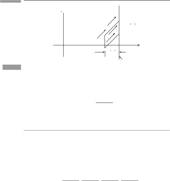
Suppose, more generally, that the particles had a y component of velocity in O¯ as well. Then the dashed line in Fig. 4.3 encloses all and only those particles that cross A in S in
87 |
4.2 Dust : the number–flux vector N |
Figure 4.3
y 
A = y z
x
υ x t
The general situation for flux: only the x-component of the velocity carries particles across a surface of constant x.
the time ¯t. This is a ‘parallelepiped’, whose volume is the area of its base times its height. But its height – its extent in the x direction – is just vx¯ ¯t. Therefore we get
(flux)x¯ |
= |
nvx¯ |
|
. |
(4.3) |
|
√(1 |
− |
v2) |
||||
|
|
|
|
|
|
|
The number–flux four-vector
N
Consider the vector N defined by
|
|
|
|
|
|
N = nU, |
|
|
|
|
|
|
(4.4) |
|||
|
|
|
|
|
|
|
|
|
|
|
O |
in which the particles have a |
||||
where U is the four-velocity of the particles. In a frame ¯ |
||||||||||||||||
velocity (vx, vy, vz), we have |
|
|
|
|
|
|
|
|
|
|
|
|
|
|
||
U→¯ |
|
√(1 1 |
v2) |
, |
√(1vx |
v2) |
, |
√(1vy |
v2) |
, |
√(1vz |
v2) |
. |
|
||
O |
|
− |
|
|
|
− |
|
|
|
− |
|
|
− |
|
|
|
It follows that |
√(1 n v2) |
, √(1 |
|
v2) |
, √(1 |
|
v2) , |
√(1 |
v2) . |
(4.5) |
||||||
N→¯ |
|
|
||||||||||||||
|
|
|
|
|
nvx |
|
|
nvy |
|
|
nvz |
|
|
|
||
O |
|
− |
|
|
|
− |
|
|
|
− |
|
|
− |
|
|
|
Thus, in any frame, the time component of N is the number density and the spatial components are the fluxes across surfaces of the various coordinates. This is a very important conceptual result. In Galilean physics, number density was a scalar, the same in all frames (no Lorentz contraction), while flux was quite another thing: a three-vector that was frame dependent, since the velocities of particles are a frame-dependent notion. Our relativistic approach has unified these two notions into a single, frame-independent four-vector. This