


88 |
Perfect fluids in special relativity |
is progress in our thinking, of the most fundamental sort: the union of apparently disparate notions into a single coherent one.
It is worth reemphasizing the sense in which we use the word ‘frame-independent’.
The vector N is a geometrical object whose existence is independent of any frame; as a tensor, its action on a one-form to give a number is independent of any frame. Its components do of course depend on the frame. Since prerelativity physicists regarded the flux as a three-vector, they had to settle for it as a frame-dependent vector, in the following sense. As a three-vector it was independent of the orientation of the spatial axes in the same sense that four-vectors are independent of all frames; but the flux threevector is different in frames that move relative to one another, since the velocity of the particles is different in different frames. To the old physicists, a flux vector had to be defined relative to some inertial frame. To a relativist, there is only one four-vector, and the frame dependence of the older way of looking at things came from concen-
trating only on a set of three of the four components of N. This unification of the Galilean frame-independent number density and frame-dependent flux into a single frame-
independent four-vector N is similar to the unification of ‘energy’ and ‘momentum’ into four-momentum.
One final note: it is clear that
N · N = −n2, n = (−N · N)1/2. |
(4.6) |
Thus, n is a scalar. In the same way that ‘rest mass’ is a scalar, even though energy and ‘inertial mass’ are frame dependent, here we have that n is a scalar, the ‘rest density’, even though number density is frame dependent. We will always define n to be a scalar number equal to the number density in the MCRF. We will make similar definitions for pressure, temperature, and other quantities characteristic of the fluid. These will be discussed later.
4.3 O n e - f o r m s a n d s u r fa ce s
Number density as a timelike flux
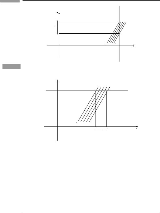
We can complete the above discussion of the unity of number density and flux by realizing that number density can be regarded as a timelike flux. To see this, let us look at the flux across x surfaces again, this time in a spacetime diagram, in which we plot only ¯t and x¯ (Fig. 4.4). The surface S perpendicular to x¯ has the world line shown. At any time ¯t it is just one point, since we are suppressing both y¯ and z¯. The world lines of those particles that go through S in the time ¯t are also shown. The flux is the number of world lines that cross S in the interval ¯t = 1. Really, since it is a two-dimensional surface, its ‘world path’ is three-dimensional, of which we have drawn only a section. The flux is the number of world lines that cross a unit ‘volume’ of this three-surface: by volume we of course
89 |
4.3 One-forms and surfaces |
|
|
|
|
|
t |
|
|
|
|
|
t |
|
|
Particles |
x |
Figure 4.4 |
¯ |
|
Fig. 4.2 in a spacetime diagram, with the y direction suppressed. |
||
t |
|
|
|
Particles |
|
x |
x |
|
|
Figure 4.5 |
¯ |
= |
const. |
|
Number density as a flux across surfaces t |
|
mean a cube of unit side, ¯t = 1, y¯ = 1, z¯ = 1. So we can define a flux as the number of world lines crossing a unit three-volume. There is no reason we cannot now define this three-volume to be an ordinary spatial volume x¯ = 1, y¯ = 1, z¯ = 1, taken at some particular time ¯t. This is shown in Fig. 4.5. Now the flux is the number crossing in the interval x¯ = 1 (since y¯ and z¯ are suppressed). But this is just the number ‘contained’ in the unit volume at the given time: the number density. So the ‘timelike’ flux is the number density.
A one -form defines a surface
The way we described surfaces above was somewhat clumsy. To push our invariant picture further we need a somewhat more satisfactory mathematical representation of the surface

90 |
Perfect fluids in special relativity |
that these world lines are crossing. This representation is given by one-forms. In general, a surface is defined as the solution to some equation
|
φ(t, x, y, z) = const. |
dφ, is a normal one-form. In some sense, dφ defines the |
|
The gradient of the function φ, ˜ |
˜ |
surface φ = const., since it uniquely determines the directions normal to that surface.
˜
However, any multiple of dφ also defines the same surface, so it is customary to use the unit-normal one-form when the surface is not null:
where
|˜ d
|˜ d
|
|
n : |
= |
˜ |
| |
˜ |
| |
|
|
|
|
|
˜ |
|
|
, |
|
(4.7) |
|||
|
|
|
|
d φ/ dφ |
|
|||||
φ| |
is |
the magnitude of |
d φ : |
|
||||||
|
˜ |
|
||||||||
φ| = | ηαβ φ,α φ,β |1/2. |
(4.8) |
|||||||||
(Do not confuse n˜ with n, the number density in the MCRF: they are completely different, given, by historical accident, the same letter.)
As in three-dimensional vector calculus (e.g. Gauss’ law), we define the ‘surface element’ as the unit normal times an area element in the surface. In this case, a volume element in a three-space whose coordinates are xα , xβ , and xγ (for some particular values of α, β, and γ , all distinct) can be represented by
n˜ dxα dxβ dxγ , |
(4.9) |
and a unit volume (dxα = dxβ = dxγ = 1) is just n˜. (These dxs are the infinitesimals that we integrate over, not the gradients.)
The flux across the surface
Recall from Gauss’ law in three dimensions that the flux across a surface of, say, the electric field is just E · n, the dot product of E with the unit normal. The situation here is exactly
the same: the flux (of particles) across a surface of constant φ is |
˜ |
|
. To see this, let φ |
||||||
n, N |
|
||||||||
|
¯ |
|
|
¯ |
|
|
¯ |
|
|
|
|
|
|
|
|
dx, which is a unit normal |
|||
be a coordinate, say x. Then a surface of constant x has normal ˜ |
|
|
|
||||||
˜ ¯ → ¯ |
(0, 1, 0, 0). Then |
˜ ¯ = |
˜ ¯ |
= |
Nx¯ , which is what we have |
||||
already since dx |
O |
dx, N |
Nα (dx)α |
|
|||||
already seen is the flux across x¯ surfaces. Clearly, had we chosen φ = ¯t, then we would
have wound up with N ¯ , the number density, or flux across a surface of constant ¯t.
0
This is one of the first concrete physical examples of our definition of a vector as a
function of one-forms into real numbers. Given the vector , we can calculate the flux
N
across a surface by finding the unit-normal one-form for that surface, and contracting it
with N. We have, moreover, expressed everything frame invariantly and in a manner that
˜ separates the property of the system of particles N from the property of the surface n. All
of this will have many parallels in § 4.4 below.