9.2 T h e d e t e c t i o n o f g ra v i t a t i o n a l wa v e s

General considerations

The great progress that astronomy has made since about 1960 is due largely to the fact that technology has permitted astronomers to begin to observe in many different parts of the electromagnetic spectrum. Because they were restricted to observing visible light, the astronomers of the 1940s could have had no inkling of such diverse and exciting phenomena as quasars, pulsars, black holes in X-ray binaries, giant black holes in galactic centers, gamma-ray bursts, and the cosmic microwave background radiation. As technology has progressed, each new wavelength region has revealed unexpected and important information. Most regions of the electromagnetic spectrum have now been explored at some level of sensitivity, but there is another spectrum which is as yet completely untouched: the gravitational wave spectrum.

As we shall see in § 9.5 below, nearly all astrophysical phenomena emit gravitational waves, and the most violent ones (which are of course among the most interesting ones!) give off radiation in copious amounts. In some situations, gravitational radiation carries information that no electromagnetic radiation can give us. For example, gravitational waves come to us direct from the heart of supernova explosions; the electromagnetic radiation from the same region is scattered countless times by the dense material surrounding the explosion, taking days to eventually make its way out, and in the process losing most of the detailed information it might carry about the explosion. As another example, gravitational waves from the Big Bang originated when the universe was perhaps only 10−25 s old; they are our earliest messengers from the beginning of our universe, and they should carry the imprint of unknown physics at energies far higher than anything we can hope to reach in accelerators on the Earth.

Beyond what we can predict, we can be virtually certain that the gravitational-wave spectrum has surprises for us; clues to phenomena we never suspected. Astronomers know that only 4% of the mass-energy of the universe is in charged particles that can emit or receive electromagnetic waves; the remaining 96% cannot radiate electromagnetically but it nevertheless couples to gravity, and some of it could turn out to radiate gravitational waves. It is not surprising, therefore, that considerable effort has been devoted to the development of sensitive gravitational-wave antennas.

The technical difficulties involved in the detection of gravitational radiation are enormous, because the amplitudes of the metric perturbations hμν that can be expected from distant sources are so small (see §§ 9.3 and 9.5 below). This is an area in which rapid advances are being made in a complex interplay between advancing technology, large investments by scientific funding agencies, and new astrophysical discoveries. This chapter reflects the situation in 2008, when sensitive detectors are in operation, even more sensitive ones are planned, but no direct detections have yet been made. The student who wants to get updated should consult the scientific literature referred to in the bibliography, § 9.6.

Purpose-built detectors are of two types: bars and interferometers.

•Resonant mass detectors. Also known as ‘bar detectors’, these are solid masses that respond to incident gravitational waves by going into vibration. The first purpose-built detectors were of this kind (Weber 1961). We shall study them below, because they can teach us a lot. But they are being phased out, because interferometers (below) have reached a better sensitivity.

•Laser interferometers. These detectors use highly stable laser light to monitor the proper distances between free masses; when a gravitational wave comes by, these distances will change – as we saw earlier. The principle is illustrated by the distance monitor described in Exer. 9, § 9.7. Very large-scale interferometers (Hough and Rowan 2000) are now being operated by a number of groups: LIGO in the USA (two 4-km detectors and a third that is 2 km long), VIRGO in Italy (3 km), GEO600 in Germany (600 m), and TAMA300 in Japan (300 m). These monitor the changes in separation between two pairs of heavy masses, suspended from supports that isolate the masses from outside vibrations. This approach has produced the most sensitive detectors to date, and is likely to produce the first detections. A very sensitive dedicated array of spacecraft, called LISA, is also planned. We will have much more to say about these detectors below.

Other ways of detecting gravitational waves are also being pursued.

•Spacecraft tracking. This principle has been used to search for gravitational waves using the communication data between Earth and interplanetary spacecraft (Armstrong 2006). By comparing small fluctuations in the round-trip time of radio signals sent to spacecraft, we try to identify gravitational waves. The sensitivity of these searches is not very high, however, because they are limited by the stability of the atomic clocks that are used for the timing and by delays caused by the plasma in the solar wind.

•Pulsar timing. Radio astronomers search for small irregularities in the times of arrival of signals from pulsars. Pulsars are spinning neutron stars that emit strong directed beams of radio waves, apparently because they have ultra-strong magnetic fields that are not aligned with the axis of rotation. Each time a magnetic pole happens to point toward Earth, the beamed emission is observed as a ‘pulse’ of radio waves. As we shall see in the next chapter, neutron stars can rotate very rapidly, even hundreds of times per second. Because the pulses are tied to the rotation rate, many pulsars are intrinsically very good clocks, potentially better than man-made ones (Cordes et al. 2004), and may accordingly be used for gravitational wave detection. Special-purpose pulsar timing arrays are currently searching for gravitational waves, by looking for correlated timing irregularities that could be caused by gravitational waves passing the radio array. When the planned Square Kilometer Array (SKA) radio telescope facility is built (perhaps around 2020), radio astronomers will have a superb tool for monitoring thousands of pulsars and digging deep for gravitational wave signals. But it is certainly conceivable that timing arrays may detect gravitational waves before the ground-based interferometers do.

•Cosmic microwave background temperature perturbations. Cosmologists study the fluctuations in the cosmic microwave background temperature distribution on the sky (see Ch. 12) for telltale signatures of gravitational waves from the Big Bang. The effect is difficult to measure, but it may come within reach of the Planck spacecraft, due for launch in 2009.

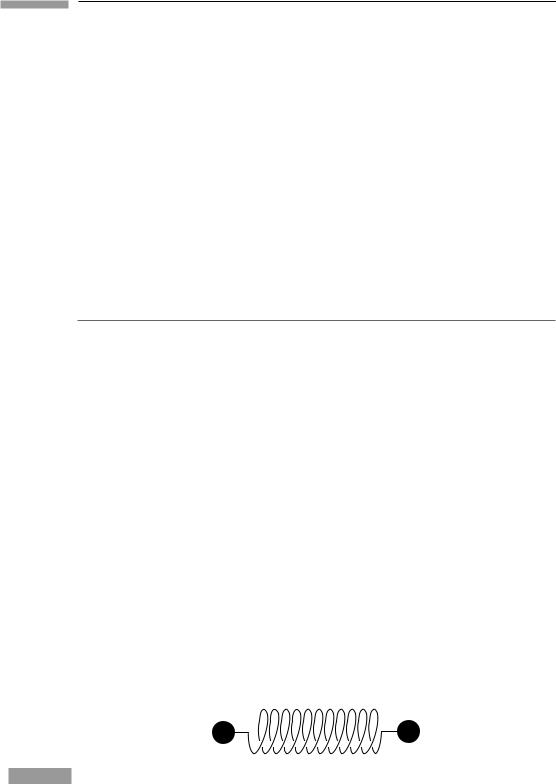
(1) A free particle remains at rest in the TT coordinates. This means that a local inertial frame at rest at, say, x1, before the wave arrives remains at rest there after the wave hits. Let its coordinates be {xα }. Suppose that the only motions in the system are those produced by the wave, i.e. that ξ = 0(l0|hμν |) l0. Then the masses’ velocities will be small as well, and Newton’s equations for the masses will apply in the local inertial frame:

where {Fj } are the components of any nongravitational forces on the masses. Because {xα } can differ from our TT coordinates {xα } only by terms of order hμν , and because x1, x1,0, and x1,00 are all of order hμν , we can use the TT coordinates in Eq. (9.37) with negligible error:

(2) The only nongravitational force on each mass is that due to the spring. Since all the motions are slow, the spring will exert a force proportional to its instantaneous proper extension, as measured using the metric. If the proper length of the spring is l, and if the gravitational wave travels in the z direction, then

Noting that the factor (x2 − x1) multiplying hTTxx can be replaced by l0 without changing the equation to the required order of accuracy, we can solve this to give

correct to first order in hTTxx . This is the fundamental equation governing the response of the detector to the gravitational wave. It has the simple form of a forced, damped harmonic oscillator. The forcing term is the tidal acceleration produced by the gravitational wave, as

given in Eq. (9.28a), although our derivation started with the proper length computation in Eq. (9.24). This shows again the self-consistency of the two approaches to understanding the action of a gravitational wave on matter. An alternative derivation of this result using the equation of geodesic deviation may be found in Exer. 21, § 9.7. The generalization to waves incident from other directions is dealt with in Exer. 22, § 9.7.

We might use a detector of this sort as a resonant detector for sources of gravitational radiation of a fixed frequency (e.g. pulsars or close binary stars). (It can also be used to detect bursts – short wave packets of broad-spectrum radiation – but we will not discuss detecting those.) Suppose that the incident wave has the form

(Of course, the general initial-value solution for ξ will also contain transients, which damp away on a timescale 1/γ .) The energy of oscillation of the detector is, to lowest order in hTTxx ,

For a detector that was at rest before the wave arrived, we have x1,0 = −x2,0 = −ξ,0/2 (see Exer. 23, § 9.7), so that

The mean value of this is its average over one period, 2π/ :

We shall always use angle brackets to denote time averages.

If we wish to detect a specific source whose frequency is known, then we should adjust ω0 to equal for maximum response (resonance), as we see from Eq. (9.48). In this case the amplitude of the response will be

The ratio /γ is related to what is usually called the quality factor Q of an oscillator, where 1/Q is defined as the average fraction of the energy of the undriven oscillator that it loses (to friction) in one radian of oscillation (see Exer. 25, § 9.7):

What numbers are realistic for laboratory detectors? Most such detectors are massive cylindrical bars in which the ‘spring’ is the elasticity of the bar when it is stretched along its axis. When waves hit the bar broadside, they excite its longitudinal modes of vibration. The first detectors, built by Joseph Weber of the University of Maryland in the 1960s, were aluminum bars of mass 1.4 × 103 kg, length l0 = 1.5 m, resonant frequency ω0 = 104 s−1, and Q about 105. This means that a strong resonant gravitational wave of A = 10−20 (see § 9.3 below) will excite the bar to an energy of the order of 10−20 J. The resonant amplitude given by Eq. (9.54) is only about 10−15 m, roughly the diameter of an atomic nucleus! Many realistic gravitational waves will have amplitudes many orders of magnitude smaller than this, and will last for much too short a time to bring the bar to its full resonant amplitude.

B ar detectors in operation

When trying to measure such tiny effects, there are in general two ways to improve things: one is to increase the size of the effect, the other is to reduce any extraneous disturbances that might obscure the measurement. And then we have to determine how best to make the measurement. The size of the effect is controlled by the amplitude of the wave, the length of the bar, and the Q-value of the material. We can’t control the wave’s amplitude, and unfortunately extending the length is not an option: realistic bars may be as long as 3 m, but longer bars would be much harder to isolate from external disturbances. In order to achieve high values of Q, some bars have actually been made of single crystals, but it is hard to do better than that. Novel designs, such as spherical detectors that respond efficiently to waves from any direction, can increase the signal somewhat, but the difficulty of making bars intrinsically more sensitive is probably the main reason that they are not the detector of choice at the moment.

The other issue in detection is to reduce the extraneous noise. For example, thermal noise in any oscillator induces random vibrations with a mean energy of kT, where T is the absolute temperature and k is Boltzmann’s constant,

k = 1.38 × 10−23 J/K.

In our example, this will be comparable to the energy of excitation if T is room temperature ( 300 K). But we chose a very optimistic wave amplitude. To detect reliably a wave with an amplitude ten times smaller would require a temperature 100 times smaller. For this reason, bar detectors in the 1980s began to change from room-temperature operation to

cryogenic operation at around 3K. The coldest, and most sensitive, bar operating today is the Auriga bar, which goes below 100 mK.

Other sources of noise, such as vibrations from passing vehicles and everyday seismic disturbances, could be considerably larger than thermal noise, so the bar has to be very carefully isolated. This is done by hanging it from a support so that it forms a pendulum with a low resonant frequency, say 1 Hz. Vibrations from the ground may move the top attachment point of the pendulum, but little of this is transmitted through to the bar at frequencies above the pendulum frequency: pendulums are good low-pass mechanical filters. In practice, several sequential pendulums may be used, and the hanging frame is further isolated from vibration by using absorbing mounts.

How do resonant detectors measure such small disturbances? The measuring apparatus is called the transducer. Weber’s original aluminum bar was instrumented with strain detectors around its waist, where the stretching of the metal is maximum. Other groups have tried to extract the energy of vibration from the bar into a transducer of very small mass that was resonant at the same frequency; if the energy extraction was efficient, then the transducer’s amplitude of oscillation would be much larger. The most sensitive readout schemes involve ultra-low-noise low-temperature superconducting devices called SQUIDs.

We have confined our discussion to on-resonance detection of a continuous wave, in the case when there are no motions in the detector. If the wave comes in as a burst with a wide range of frequencies, where the excitation amplitude might be smaller than the broad-band noise level, then we have to do a more careful analysis of their sensitivity, but the general picture does not change. One difficulty bars encounter with broadband signals is that it is difficult for them in practice (although not impossible in principle) to measure the frequency components of a waveform very far from their resonant frequencies, which normally lie above 600 Hz. Since most strong sources of gravitational waves emit at lower frequencies, this is a serious problem. A second difficulty is that, to reach a sensitivity to bursts of amplitude around 10−21 (which is the level that interferometers reached in 2005), bars need to conquer the so-called quantum limit. At these small excitations, the energy put into the vibrations of the bar by the wave is below one quantum (one phonon) of excitation of the resonant mode being used to detect them. The theory of how to detect below the quantum limit – of how to manipulate the Heisenberg uncertainty relation in a macroscopic object like a bar – is fascinating. But the challenge has not yet been met in practice, and is therefore another serious problem that bars face. For more details on all of these issues, see Misner et al. (1973), Smarr (1979), or Blair (1991).

The severe technical challenges of bar detectors come fundamentally from their small size: any detector based on the resonances of a metal object cannot be larger than a few meters in size, and that seriously limits the size of the tidal stretching induced by a gravitational wave. Laser interferometer detectors are built on kilometer scales (and in space, on scales of millions of kilometers). They therefore have an inherently larger response and are consequently able to go to a higher sensitivity before they become troubled by quantum, vibration, and thermal noise. The inherent difficulties faced by bars have led to a gradual reduction in research funding for bar detectors during the period after 2000, as interferometers have steadily improved and finally surpassed the sensitivity of the best bars. After 2010 it seems unlikely that any bar detectors will remain in operation.