11 Schwarzschild geometry and black holes

11.1 Tra j e c t o r i e s i n t h e S c h wa r z s c h i l d s p a ce t i m e

The ‘Schwarzschild geometry’ is the geometry of the vacuum spacetime outside a spherical star. It is determined by one parameter, the mass M, and has the line element

in the coordinate system developed in the previous chapter. Its importance is not just that it is the gravitational field of a star: we shall see that it is also the geometry of the spherical black hole. A careful study of its timelike and null geodesics – the paths of freely moving particles and photons – is the key to understanding the physical importance of this metric.

Black holes in Newtonian gravity

Before we embark on the study of fully relativistic black holes, it is well to understand that the physics is not really exotic, and that speculations on analogous objects go back two centuries. It follows from the weak equivalence principle, which was part of Newtonian gravity, that trajectories in the gravitational field of any body depend only on the position and velocity of the particle, not its internal composition. The question of whether a particle can escape from the gravitational field of a body is, then, only an issue of velocity: does it have the right escape velocity for the location it starts from. For a spherical body like a star, the escape velocity depends only on how far one is from the center of the body.

Now, a star is visible to us because light escapes from its surface. As long ago as the late 1700’s, the British physicist John Michell and the French mathematician and physicist Pierre Laplace speculated (independently) on the possibility that stars might exist whose escape velocity was larger than the speed of light. At that period in history, it was popular to regard light as a particle traveling at a finite speed. Michell and Laplace both understood that if nature were able to make a star more compact than the Sun, but with the same mass, then it would have a larger escape velocity. It would therefore be possible in principle to make it compact enough for the escape velocity to be the velocity of light. The star would then be dark, invisible. For a spherical star, this is a simple computation. By conservation of energy, a particle launched from the surface of a star with mass M and radius R will

Conserved quantities

We begin our study of relativistic black holes by examining the trajectories of particles. This will allow us eventually to see whether light rays are trapped or can escape.

We have seen (Eq. (7.29) and associated discussion) that when a spacetime has a certain symmetry, then there is an associated conserved momentum component for trajectories. Because our space has so many symmetries – time independence and spherical symmetry – the values of the conserved quantities turn out to determine the trajectory completely. We shall treat ‘particles’ with mass and ‘photons’ without mass in parallel.

Time independence of the metric means that the energy −p0 is constant on the trajectory. For massive particles with rest mass m =0, we define the energy per unit mass (specific

˜

energy) E, while for photons we use a similar notation just for the energy E:

Independence of the metric of the angle φ about the axis implies that the angular momen-

˜

tum pφ is constant. We again define the specific angular momentum L for massive particles and the ordinary angular momentum L for photons:

Because of spherical symmetry, motion is always confined to a single plane, and we can choose that plane to be the equatorial plane. Then θ is constant (θ = π/2) for the orbit, so dθ /dλ = 0, where λ is any parameter on the orbit. But pθ is proportional to this, so it also vanishes. The other components of momentum are:

The equation for a photon’s pr should be regarded as defining the affine parameter λ. The equation p · p = −m2 implies

particle :

Types of orbi ts

Both equations have the same general form, and we define the effective potentials

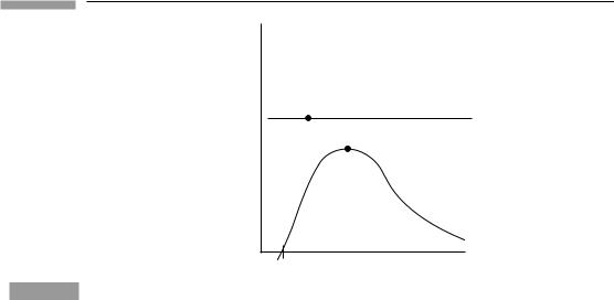
Their typical forms are plotted in Figs. 11.1 and 11.2, in which various points have been labeled and possible trajectories drawn (dotted lines).

Both Eq. (11.11) and Eq. (11.12) imply that, since the left side is positive or zero, the energy of a trajectory must not be less than the potential V. (Here and until Eq. (11.17)

˜ ˜

we will take E and V to refer to E and V as well, since the remarks for the two cases are

identical.) So for an orbit of given E, the radial range is restricted to those radii for which V is smaller than E. For instance, consider the trajectory which has the value of E indicated by point G (in either diagram). If it comes in from r = ∞, then it cannot reach smaller r than where the dotted line hits the V2 curve, at point G. Point G is called a turning point. At G, since E2 = V2 we must have (dr/dλ)2 = 0, from Eq. (11.12). Similar conclusions apply to Eq. (11.11). To see what happens here we differentiate Eqs. (11.11) and (11.12). For particles, differentiating the equation

These are the analogs in relativity of the equation ma = − φ,

where φ is the potential for some force. If we now look again at point G, we see that the radial acceleration of the trajectory is outwards, so that the particle (or photon) comes in to the minimum radius, but is accelerated outward as it turns around, and so it returns to r = ∞. This is a ‘hyperbolic’ orbit – the analog of the orbits which are true hyperbolae in Newtonian gravity.