


46 |
Vector analysis in special relativity |
t 
→
e0
→
e1
|
|
|
|
x |
|
|
|
|
O¯ |
|
O |
|
Figure 2.4 |
The basis vectors of |
are not ‘perpendicular’ (in the Euclidean sense) when drawn in |
||
|
|
, but |
they are orthogonal with respect to the dot product of Minkowski spacetime.
so that, in particular, e0¯ · e1¯ = 0. Look at this in the spacetime diagram of O, Fig. 2.4: The two vectors certainly are not perpendicular in the picture. Nevertheless, their scalar product is zero. The rule is that two vectors are orthogonal if they make equal angles with the 45◦ line representing the path of a light ray. Thus, a vector tangent to the light ray is orthogonal to itself. This is just another way in which SR cannot be ‘visualized’ in terms of notions we have developed in Euclidean space.
Example
The four-velocity U of a particle is just the time basis vector of its MCRF, so from Eq. (2.27) we have
· = −
U U 1. (2.28)
2.6 A p p l i c a t i o n s
Four-velocity and acceleration as derivatives
Suppose a particle makes an infinitesimal displacement dx, whose components in O are (dt, dx, dy, dz). The magnitude of this displacement is, by Eq. (2.24), just −dt2 + dx2 + dy2 + dz2. Comparing this with Eq. (1.1), we see that this is just the interval, ds2:
ds2 = dx · dx. |
(2.29) |
Since the world line is timelike, this is negative. This led us (Eq. (1.9)) to define the proper time dτ by
(dτ )2 = −dx · dx. |
(2.30) |
47 |
|
2.6 Applications |
|
|
|
|
|
|
Now consider the vector dx/dτ , where dτ is the square root of Eq. (2.30) (Fig. 2.5). This vector is tangent to the world line since it is a multiple of dx. Its magnitude is
dx · dx = dx · dx = −1. dτ dτ (dτ )2
It is therefore a timelike vector of unit magnitude tangent to the world line. In an MCRF,
dx −→ (dt, 0, 0, 0).
MCRF dτ = dt
so that
dx −→ (1, 0, 0, 0)
dτ MCRF
or
dx = (e0)MCRF.
dτ
This was the definition of the four-velocity. So we have the useful expression
U |
= |
|
(2.31) |
|||
|
dx/dτ . |
|||||
Moreover, let us examine |
|
|
, |
|
||
dU |
|
|||||
= |
d2x |
|
|
|||
|
dτ |
dτ 2 |
|
|
||
which is some sort of four-acceleration. First we differentiate Eq. (2.28) and use Eq. (2.26):
|
d |
|
|
dU |
||
|
|
(U · U) = 2U · |
|
. |
||
dτ |
dτ |
|||||
But since U · U = −1 is a constant we have |
|
|
|
|||
|
|
U · |
dU |
= 0. |
|
|
|
|
dτ |
|
|
||
t |
|
|
|
|
||
|
|
|
|
→ |
|
|
|
|
|
|
dx |
|
|
x
|
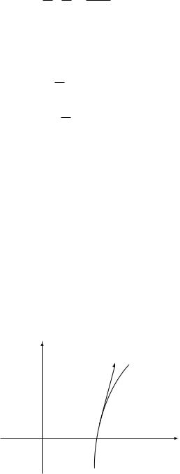
Figure 2.5 |
|
|
The infinitesimal displacement vector dx tangent to a world line. |

48 |
Vector analysis in special relativity |
Since, in the MCRF, U has only a zero component, this orthogonality means that
dU −→ (0, a1, a2, a3).
dτ MCRF
This vector is defined as the acceleration four-vector a:
= |
dτ |
U |
· |
= |
0. |
(2.32) |
a |
dU , |
a |
|
Exer. 19, § 2.9, justifies the name ‘acceleration’.
Energy and momentum
Consider a particle whose momentum is p. Then |
|
|
|||
p p |
m2U |
· |
U |
m2. |
(2.33) |
· = |
|
|
= − |
|
|
But
p · p = −E2 + (p1)2 + (p2)2 + (p3)2.
Therefore,
|
|
3 |
|
|
|
|
|
(pi)2. |
|
E2 = m2 + |
(2.34) |
|||
|
|
i=1 |
|
|
This is the familiar expression for the total energy of a particle. |
||||
O |
|
|
|
not necessarily equal to the |
Suppose an observer ¯ moves with four-velocity Uobs |
||||
particle’s four-velocity. Then |
|
|
|
|
· |
Uobs |
= · ¯ |
|
|
p |
p |
e0, |
|
|
where e0¯ is the basis vector of the frame of the observer. In that frame the four-momentum
has components |
|
(E¯ , p1¯ , p2¯ , p3¯ ). |
|
|||
p |
|
|
||||
→ |
|
|
|
|
|
|
|
¯ |
|
|
|
|
|
|
O |
|
|
|
|
|
Therefore, we obtain, from Eq. (2.26), |
|
|
|
|
|
|
|
|
|
|
|
|
|
|
− · |
Uobs |
= |
E.¯ |
(2.35) |
|
|
p |
|
||||
This is an important equation. It says that the energy of the particle relative to the observer,
¯ ·
E, can be computed by anyone in any frame by taking the scalar product p Uobs. This is called a ‘frame-invariant’ expression for the energy relative to the observer. It is almost always helpful in calculations to use such expressions.