


3 Tensor analysis in special relativity
3.1 T h e m e t r i c t e n s o r
|
|
|
|
|
|
|
|
|
|
|
{ |
|
} |
of some frame |
O |
: |
|
|
|
|
|
|
A and B on the basis e |
|
|
|
|||||||
Consider the representation of two vectors |
|
|
|
|
|
α |
|
|
|
|
||||||
|
|
|
|
|
|
α |
|
|
|
β |
|
|
|
|
|
|
A |
= |
Aα e , |
B |
= |
Bβ e . |
|
|
|
|
|
||||||
|
|
|
|
|
|
|
|
|
|
|
|
|
|
|||
Their scalar product is |
|
|
|
|
|
|
|
|
|
|
|
|
|
|
|
|
A |
· |
B |
= |
(Aα |
|
· |
|
β |
|
|
|
|
|
|
||
|
|
|
|
|
|
|
|
|
|
|
||||||
|
|
|
|
eα ) |
|
(B eβ ). |
|
|
|
|
|
|||||
(Note the importance of using different indices α and β to distinguish the first summation from the second.) Following Exer. 34, § 2.9, we can rewrite this as
|
|
|
|
α |
|
β |
|
A |
· |
B |
= |
Aα Bβ (e |
e |
|
), |
|
|
|
· |
|
|
which, by Eq. (2.27), is
|
· |
= |
Aα Bβ η |
αβ |
. |
(3.1) |
A |
B |
|
|
This is a frame-invariant way of writing
−A0B0 + A1B1 + A2B2 + A3B3.
The numbers ηαβ are called ‘components of the metric tensor’. We will justify this name later. Right now we observe that they essentially give a ‘rule’ for associating with two
vectors A and B a single number, which we call their scalar product. The rule is that the number is the double sum Aα Bβ ηαβ . Such a rule is at the heart of the meaning of ‘tensor’, as we now discuss.
3.2 D e fi n i t i o n o f t e n s o r s
We make the following definition of a tensor:
A tensor of type N0 is a function of N vectors into the real numbers, which is linear in each of its N arguments.

57 |
|
|
|
3.2 Definition of tensors |
|
|
|
|
|||||||
|
|
|
|
|
|
|
|
|
|
|
|
|
|
|
|
|
Let us see what this definition means. For the moment, we will just accept the notation |
0 |
; |
||||||||||||
|
|||||||||||||||
|
|
|
|
|
|
|
|
|
|
|
|
|
|
N |
|
|
|
|
|
|
|
|
|
|
|
|
|
|
3.1), |
||
|
its justification will come later in this chapter. The rule for the scalar product, Eq. ( |
|
|
||||||||||||
|
satisfies our definition of a |
0 |
|
|
|
|
|
|
|
A and B, and |
|||||
|
2 tensor. It is a rule which takes two vectors, |
|
|
|
|||||||||||
|
produces a single real |
number A B. To say that it is linear in its arguments means what is |
|||||||||||||
|
|
|
· |
|
|
|
|
|
|
|
|
|
|
||
|
proved in Exer. 34, § 2.9. Linearity on the first argument means |
|
|
|
|||||||||||
|
|
|
and |
(α |
|
· |
= |
|
· |
|
|
(3.2) |
|||
|
|
|
|
|
A) |
B |
|
α(A B), |
|
|
|
|
|||
|
|
|
|
|
(A B) |
|
C A C B C, |
|
|
|
|||||
|
|
|
|
|
+ |
· = · |
+ |
· |
|
|
|
|
|||
|
while linearity on the second argument means |
|
|
|
|
|
|
||||||||
|
|
|
|
|
· (βB) = β( · |
|
|
|
|
|
|
||||
|
|
|
|
A |
· (B + |
|
A |
B), |
|
|
|
|
|
|
|
|
|
|
|
|
|
= |
· + · |
|
|
|
|
||||
|
|
|
|
A |
C) |
|
A |
B |
A |
C. |
|
|
|
|
|
This definition of linearity is of central importance for tensor algebra, and the student should study it carefully.
To give concreteness to this notion of the dot product being a tensor, we introduce a name and notation for it. We let g be the metric tensor and write, by definition,
g( |
= |
· |
(3.3) |
A, B) : |
A |
B. |
Then we regard g( , ) as a function which can take two arguments, and which is linear in that
|
+ |
) = |
) + |
|
(3.4) |
g(αA |
|
βB, C |
α g(A, C |
β g(B, C), |
and similarly for the second argument. The value of g on two arguments, denoted by
g(A, B), is their dot product, a real number.
Notice that the definition of a tensor does not mention components of the vectors. A tensor must be a rule which gives the same real number independently of the reference frame in which the vectors’ components are calculated. We showed in the previous chapter that Eq. (3.1) satisfies this requirement. This enables us to regard a tensor as a function of the vectors themselves rather than of their components, and this can sometimes be helpful conceptually.
Notice that an ordinary function of position, f (t, x, y, z), is a real-valued function of no
vectorsat all. It is therefore classified as a 00 tensor.
A side on the us age of the term ‘function’
The most familiar notion of a function is expressed in the equation
y = f (x),
where y and x are real numbers. But this can be written more precisely as: f is a ‘rule’ (called a mapping) which associates a real number (symbolically called y, above) with another real number, which is the argument of f (symbolically called x, above). The function itself is not f (x), since f (x) is y, which is a real number called the ‘value’ of the

58 |
|
Tensor analysis in special relativity |
|||
|
|
|
|
|
|
|
function. The function itself is f , which we can write as f ( |
) in order to show that it has |
|||
|
|||||
|
one argument. In algebra this seems like hair-splitting since we unconsciously think of x |
||||
|
and y as two things at once: they are, on the one hand, specific real numbers and, on the |
||||
|
other hand, names for general and arbitrary real numbers. In tensor calculus we will make |
||||
|
|
A and B are specific vectors, A B is a specific real number, and g |
|||
|
this distinction explicit: |
|
· |
|
|
|
|
|
A B with A and B. |
||
|
is the name of the function that associates · |
|
|
||
Components of a tensor
Just like a vector, a tensor has components. They are defined as:
The components in a frame O of a tensor of type 0 are the values of the function when its arguments
N
are the basis vectors {eα } of the frame O.
Thus we have the notion of components as frame-dependent numbers (frame-dependent because the basis refers to a specific frame). For the metric tensor, this gives the components as
g(eα , eβ ) = eα · eβ = ηαβ . |
(3.5) |
So the matrix ηαβ that we introduced before is to be thought of as an array of the components of g on the basis. In another basis, the components could be different. We will have many more examples of this later. First we study a particularly important class of tensors.
3.3 T h e 01 t e n s o r s : o n e - f o r m s
A tensor of the type 01 is called a covector, a covariant vector, or a one-form. Often these names are used interchangeably, even in a single text-book or reference.
General properties
Let an arbitrary one-form be called p˜. (We adopt the notation that ˜ above a symbol denotes a one-form, just as above a symbol denotes a vector.) Then p˜, supplied with one vector
˜ |
|
˜ |
|
A) is a real number. Suppose q is another one-form. Then |
|
argument, gives a real number: p( |
|
|
we can define |
r˜ = αp˜, |
|
|
||
|
s˜ = p˜ + q˜, |
(3.6a) |

59 |
3.3 The 10 tensors: one-forms |
to be the one-forms that take the following values for an argument A:
s( |
|
|
+ |
|
|
|
r˜( ˜ |
= |
|
||||
˜ |
A) |
= ˜ |
|
|
(3.6b) |
|
|
p(A) |
q(A), |
|
|||
|
A) |
αp(A). |
|
|
||
With these rules, the set of all one-forms satisfies the axioms for a vector space, which accounts for their other names. This space is called the ‘dual vector space’ to distinguish it
from the space of all vectors such as A.
When discussing vectors we relied heavily on components and their transformations. Let us look at those of p˜. The components of p˜ are called pα :
pα := p˜(eα ). |
(3.7) |
Any component with a single lower index is, by convention, the component of a one-form;
|
|
|
|
|
|
˜ |
A) is |
|
an upper index denotes the component of a vector. In terms of components, p( |
|
|||||||
˜ |
A) |
|
p(Aα |
|
|
|
||
|
= ˜ |
|
|
|
||||
p( |
|
|
|
eα ) |
|
|
||
|
|
= Aα p˜(eα ), |
|
|
||||
˜ |
A) |
= |
Aα p . |
|
(3.8) |
|||
p( |
|
|
α |
|
|
|
||
The second step follows from the linearity which is the heart of the definition we gave of a
˜ |
A) is easily found to be the sum A0 |
+ |
1 |
|
+ |
|
2 |
|
+ |
3 |
tensor. So the real number p( |
p0 A |
|
p1 |
|
A |
|
p2 |
|
A p3. |
|
|
|
|
|
|
|
A and p, and |
||||
Notice that all terms have plus signs: this operation is called contraction of |
|
|
˜ |
|||||||
is more fundamental in tensor analysis than the scalar product because it can be performed between any one-form and vector without reference to other tensors. We have seen that two vectors cannot make a scalar (their dot product) without the help of a third tensor, the
metric. |
|
{ |
¯ } |
|
|
|
|
|
|
|
|
|
|
|
|
|
|
|
|
˜ |
|
are |
|
|
|
|
|
|
|
|
|
|
|||||||
The components of p on a basis |
|
eβ |
|
|
|
|
|
|
|
|
|
|
|||||||
p |
¯ |
: |
|
p(e |
|
¯ |
) |
|
p( α |
|
eα ) |
|
|||||||
|
|
= ˜ |
|
|
= ˜ |
|
|
|
¯ |
|
|
||||||||
|
β |
|
|
α |
|
β |
|
|
|
|
|
|
β |
|
|
pα . |
(3.9) |
||
|
|
= |
|
|
p(eα ) |
= |
α |
¯ |
|||||||||||
|
|
|
|
¯ ˜ |
|
|
|
|
|
|
|||||||||
|
|
|
|
|
|
β |
|
|
|
|
|
|
|
|
|
β |
|
|
|
Comparing this with |
|
|
|
e |
|
|
|
|
|
α |
|
|
eα , |
|
|
|
|
|
|
|
|
|
|
¯ |
= |
|
|
|
|
|
|
|
|||||||
|
|
|
|
|
|
¯ |
|
|
|
|
|
|
|||||||
|
|
|
|
β |
|
|
|
|
|
β |
|
|
|
|
|
|
|
||
we see that components of one-forms transform in exactly the same manner as basis vectors and in the opposite manner to components of vectors. By ‘opposite’, we mean using the
inverse transformation. This use of the inverse guarantees that Aα pα is frame independent |
||
A and one-form p. This is such an important observation that we shall prove |
||
for any vector |
˜ |
|
it explicitly: |
|
|
|
Aα¯ pα¯ = ( α¯ β Aβ )( μα¯ pμ), |
(3.10a) |
|
= μα¯ α¯ β Aβ pμ, |
(3.10b) |
|
= δμβ Aβ pμ, |
(3.10c) |
|
= Aβ pβ . |
(3.10d) |

60 |
Tensor analysis in special relativity |
(This is the same way in which the vector Aα eα is kept frame independent.) This inverse transformation gives rise to the word ‘dual’ in ‘dual vector space’. The property of transforming with basis vectors gives rise to the co in ‘covariant vector’ and its shorter form ‘covector’. Since components of ordinary vectors transform oppositely to basis vectors (in order to keep Aβ eβ frame independent), they are often called ‘contravariant’ vectors. Most of these names are old-fashioned; ‘vectors’ and ‘dual vectors’ or ‘one-forms’ are the modern names. The reason that ‘co’ and ‘contra’ have been abandoned is that they mix up two very different things: the transformation of a basis is the expression of new vectors in terms of old ones; the transformation of components is the expression of the same object in terms of the new basis. It is important for the student to be sure of these distinctions before proceeding further.
B asis one -forms
Since the set of all one-forms is a vector space, we can use any set of four linearly independent one-forms as a basis. (As with any vector space, one-forms are said to be linearly independent if no nontrivial linear combination equals the zero one-form. The zero oneform is the one whose value on any vector is zero.) However, in the previous section we have already used the basis vectors {eα } to define the components of a one-form. This suggests that we should be able to use the basis vectors to define an associated one-form basis {ω˜ α , α = 0, . . . , 3}, which we shall call the basis dual to {eα }, upon which a one-form has the components defined above. That is, we want a set {ω˜ α } such that
p˜ = pα ω˜ α . |
(3.11) |
(Notice that using a raised index on ω˜ α permits the summation convention to operate.) The {ω˜ α } are four distinct one-forms, just as the {eα } are four distinct vectors. This equation A and one-form p:
must imply Eq. (3.8) for any vector |
|
|
|
|
|
|
|
˜ |
|
|
p(A) |
= |
p |
α |
Aα . |
||||
|
˜ |
|
|
|
|
||||
But from Eq. (3.11) we get |
|
|
|
|
|
|
|
|
|
|
A) |
|
p |
α |
ωα (A) |
||||
p( |
= |
|
|
|
˜ |
|
|
||
˜ |
|
|
|
|
|
|
|
||
= pα ω˜ α (Aβ eβ ) = pα Aβ ω˜ α (eβ ).
(Notice the use of β as an index in the second line, in order to distinguish its summation from the one on α.) Now, this final line can only equal pα Aα for all Aβ and pα if
ω˜ α (eβ ) = δα β . |
(3.12) |
Comparing with Eq. (3.7), we see that this equation gives the βth component of the αth basis one-form. It therefore defines the αth basis one-form. We can write out these components as
61 |
3.3 The 10 tensors: one-forms |
ω˜ 0 → (1, 0, 0, 0),
O
ω˜ 1 → (0, 1, 0, 0),
O
ω˜ 2 → (0, 0, 1, 0),
O
ω˜ 3 → (0, 0, 0, 1).
O
It is important to understand two points here. One is that Eq. (3.12) defines the basis {ω˜ α } in terms of the basis {eβ }. The vector basis induces a unique and convenient oneform basis. This is not the only possible one-form basis, but it is so useful to have the relationship, Eq. (3.12), between the bases that we will always use it. The relationship, Eq. (3.12), is between the two bases, not between individual pairs, such as ω˜ 0 and e0. That is, if we change e0, while leaving e1, e2, and e3 unchanged, then in general this induces changes not only in ω˜ 0 but also in ω˜ 1, ω˜ 2, and ω˜ 3. The second point to understand is that, although we can describe both vectors and one-forms by giving a set of four components, their geometrical significance is very different. The student should not lose sight of the fact that the components tell only part of the story. The basis contains the rest of the information. That is, a set of numbers (0, 2, −1, 5) alone does not define anything; to make it into something, we must say whether these are components on a vector basis or a one-form basis and, indeed, which of the infinite number of possible bases is being used.
It remains to determine how {ω˜ α } transforms under a change of basis. That is, each frame has its own unique set {ω˜ α }; how are those of two frames related? The derivation here is analogous to that for the basis vectors. It leads to the only equation we can write down with the indices in their correct positions:
ωα¯ |
= |
α¯ ωβ . |
(3.13) |
˜ |
β ˜ |
|
This is the same as for components of a vector, and opposite that for components of a one-form.
Picture of a one -form
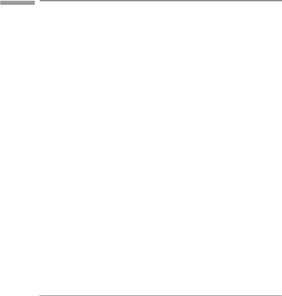
For vectors we usually imagine an arrow if we need a picture. It is helpful to have an image of a one-form as well. First of all, it is not an arrow. Its picture must reflect the fact that it maps vectors into real numbers. A vector itself does not automatically map another vector into a real number. To do this it needs a metric tensor to define the scalar product. With a different metric, the same two vectors will produce a different scalar product. So two vectors by themselves don’t give a number. We need a picture of a one-form which doesn’t depend on any other tensors having been defined. The one generally used by mathematicians is shown in Fig. 3.1. The one-form consists of a series of surfaces. The ‘magnitude’ of it is given by the spacing between the surfaces: the larger the spacing the smaller the magnitude. In this picture, the number produced when a one-form acts on a vector is the number of surfaces that the arrow of the vector pierces. So the closer their
62 |
Tensor analysis in special relativity |
Figure 3.1
(a) |
(b) |
(c) |
(a) The picture of one-form complementary to that of a vector as an arrow. (b) The value of a one-form on a given vector is the number of surfaces the arrow pierces. (c) The value of a smaller one-form on the same vector is a smaller number of surfaces. The larger the one-form, the more ‘intense’ the slicing of space in its picture.
spacing, the larger the number (compare (b) and (c) in Fig. 3.1). In a four-dimensional space, the surfaces are three-dimensional. The one-form doesn’t define a unique direction, since it is not a vector. Rather, it defines a way of ‘slicing’ the space. In order to justify this picture we shall look at a particular one-form, the gradient.
Gradient of a function is a one -form
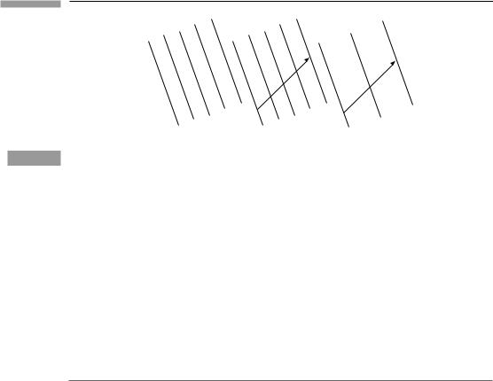
Consider a scalar field φ(x) defined at every event x. The world line of some particle (or person) encounters a value of φ at each on it (see Fig. 3.2), and this value changes from event to event. If we label (parametrize) each point on the curve by the value of proper time τ along it (i.e. the reading of a clock moving on the line), then we can express the coordinates of events on the curve as functions of τ :
[t = t(τ ), x = x(τ ), y = y(τ ), z = z(τ )].
The four-velocity has components
U → |
d t d x |
|||
|
, |
|
, . . . . |
|
dτ |
dτ |
|||
Since φ is a function of t, x, y, and z, it is implicitly a function of τ on the curve:
φ(τ ) = φ[t(τ ), x(τ ), y(τ ), z(τ )],
and its rate of change on the curve is
63
Figure 3.2
3.3 The 01 tensors: one-forms
t 
τ = 2 |
→ |
U |
τ = 1 φ(τ) = φ[t(τ), x(τ), y(τ), z(τ)]
τ = 0
x
A world line parametrized by proper time τ , and the values φ(τ ) of the scalar field φ(t, x, y, z) along it.
dφ |
= |
∂φ dt |
+ |
|
∂φ dx |
+ |
|
∂φ dy |
+ |
∂φ dz |
|
|||||||||||||
|
|
|
|
|
|
|
|
|
|
|
|
|
|
|
|
|
|
|
||||||
dτ |
|
∂t dτ |
|
∂x dτ |
|
∂y dτ |
∂z |
dτ |
|
|||||||||||||||
|
|
∂φ |
|
∂φ |
|
∂φ |
|
∂φ |
|
|||||||||||||||
|
= |
|
|
Ut + |
|
Ux |
+ |
|
|
Uy + |
|
Uz. |
(3.14) |
|||||||||||
|
|
∂t |
∂x |
|
∂y |
∂z |
||||||||||||||||||
It is clear from this that in the last equation we have devised a means of producing from
the vector U the number dφ/dτ that represents the rate of change of φ on a curve on which
U is the tangent. This number dφ/dτ is clearly a linear function of U, so we have defined
a one-form. |
|
|
|
|
|
|
|
|
|
|
|
|
|
By comparison |
with Eq. (3.8), |
we see that this one-form has |
components |
||||||||||
(∂φ/∂t, ∂φ/∂x, |
∂φ/∂y, |
∂φ/∂z). This one-form is called the gradient of φ, denoted by ˜ |
|||||||||||
|
|
→O |
∂t ∂x ∂y ∂z |
dφ: |
|||||||||
|
|
|
˜ |
|
|||||||||
|
|
|
dφ |
|
∂φ |
, |
∂φ |
, |
∂φ |
, |
∂φ |
. |
(3.15) |
|
|
|
|
|
|
|
|
||||||
It is clear that the gradient fits our definition of a one-form. We will see later how it comes about that the gradient is usually introduced in three-dimensional vector calculus as a vector.
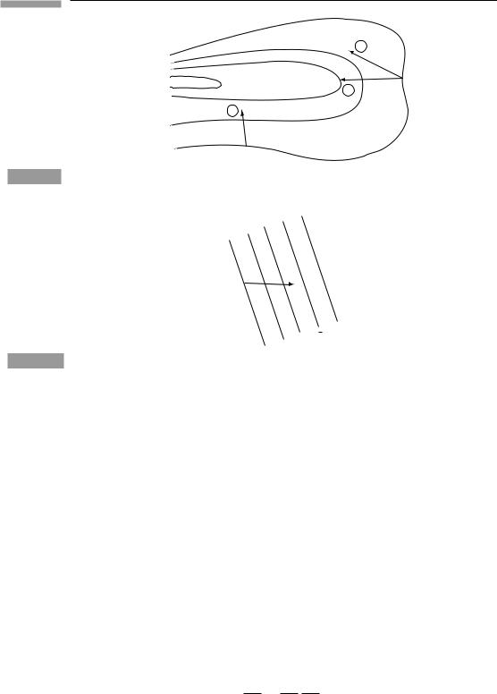
The gradient enables us to justify our picture of a one-form. In Fig. 3.3 we have drawn part of a topographical map, showing contours of equal elevation. If h is the elevation, then
˜
the gradient dh is clearly largest in an area such as A, where the lines are closest together, and smallest near B, where the lines are spaced far apart. Moreover, suppose we wanted to know how much elevation a walk between two points would involve. We would lay out on the map a line (vector x) between the points. Then the number of contours the line crossed would give the change in elevation. For example, line 1 crosses 1 12 contours, while 2 crosses two contours. Line 3 starts near 2 but goes in a different direction, winding up
|
1 |
|
|
|
|
|
dh with |
only |
2 |
contour higher. But these numbers are just h, which is the contraction of ˜ |
|||||
x : h = i |
(∂h/∂x |
) x |
i |
or the value of ˜ |
|
||
|
|
|
i |
|
dh on x (see Eq. (3.8)). |
||
|
|
|
|
|
|
||
64 |
Tensor analysis in special relativity |
Figure 3.3
Figure 3.4
|
A |
3 |
|
|
|
40 |
|
2 |
30 |
|
|
|
|
|
|
|
1 |
20 |
|
B |
|
|
|
10 |
|
|
A topographical map illustrates the gradient one-form (local contours of constant elevation). The change of height along any trip (arrow) is the number of contours crossed by the arrow.
→
V
ω
The value ω˜ (V) is 2.5.
Therefore, a one-form is represented by a series of surfaces (Fig. 3.4), and its contraction
with a vector V is the number of surfaces V crosses. The closer the surfaces, the larger ω˜ . Properly, just as a vector is straight, the one-form’s surfaces are straight and parallel. This is because we deal with one-forms at a point, not over an extended region: ‘tangent’ one-forms, in the same sense as tangent vectors.
These pictures show why we in general cannot call a gradient a vector. We would like to identify the vector gradient as that vector pointing ‘up’ the slope, i.e. in such a way that it crosses the greatest number of contours per unit length. The key phrase is ‘per unit length’. If there is a metric, a measure of distance in the space, then a vector can be associated with a gradient. But the metric must intervene here in order to produce a vector. Geometrically, on its own, the gradient is a one-form.
Let us be sure that Eq. (3.15) is a consistent definition. How do the components transform? For a one-form we must have
˜ α |
= |
β |
α |
˜ |
β |
|
|
|
(dφ) |
¯ |
¯ |
(dφ) |
|
. |
(3.16) |
||
|
|
|
|
|||||
But we know how to transform partial derivatives:
∂φ ∂φ ∂xβ
∂xα¯ = ∂xβ ∂xα¯ ,