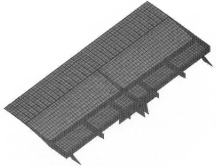
Fig. 16.3 Finite element model for a wing spoiler--top skin removed.

The finite element model, however, does not provide an exact match to experimental results. The theoretical processes are based on a numerical approximation related to the element size, the type of element used, the underlying theory, and the type of analysis performed. The modelling process involves approximations for geometry and may not reflect the true detail such as the change of the orientation of fibers during lay-up and cure. The stiffness of joints and imperfections such as the straightness of beams and flatness of panels can have considerable influence on the performance of actual structures. 5 The achievement of relevant and useful results relies on an understanding of the characteristics of the solution process and care when developing the numerical models.

16.3Finite Element Solution Process

The finite element method provides the design team with information regarding the stiffness and strength of the structure. What confidence should the design team have in the results when analyzing composite structures? Unfortunately, the answer depends, in part, on how well the method is implemented. To indicate some of the features of the finite element method, the

554 COMPOSITE MATERIALS FOR AIRCRAFT STRUCTURES

Fig. 16.4 A 1-D example to introduce FEA. A hollow tube of composite or metal is supported at its left-hand end and carries the loads shown.

one-dimensional problem shown in Figure 16.4 will be considered. The emphasis will be on explaining how the method works and how is it applied to composite materials.6

In all applications, as in this example, the development of the finite element model and completion of the analysis involves six basic steps:

Step 1. Select the type of analysis that will be executed. The selection of a full three-dimensional non-linear analysis is the most general but can lead to a model with a very large number of elements if the structure consists of thin panels. Finite elements need to be of moderate aspect ratio. The size of a threedimensional brick element will therefore be governed by the minimum dimension (usually the thickness). As a result, engineers have developed beam, plate, and shell approximations to structural behavior. These approximations reduce the dimension of the problem. For example, in the classical laminate plate theory described in Chapter 6, the in-plane strains are assumed to be constant through the thickness in planar two-dimensional analysis, and linear through-the- thickness when the response includes bending. A finite element analysis based on plate elements will use these approximations to eliminate the thickness dimension. The finite elements are planar, and the size of each element is governed by the in-plane dimensions. The implications of assuming the behavior is linear will be discussed later.

The geometry considered here is that relevant to a hollow tube. The most detailed analysis could include accurate modelling of the tube wall in three dimensions with a layer of elements for each ply, modelling of the fixed support, modelling of the change in section, and how the load is applied. A simpler analysis would model the wall using plate or shell elements with the element lying in the plane of the wall, limiting the variation of strain through the thickness to a linear distribution and eliminating the modelling of more complex behavior.

uL P~ u2 p_t

O O

I

Fig. 16.5 The rod finite element used in the analysis.

556 COMPOSITE MATERIALS FOR AIRCRAFT STRUCTURES

Set u2 equal to 1 and u 1 equal to zero. Then, from equation (16.1),

Defining a similar problem with ul equal to 1 and u2 equal to zero identifies:

Combining these results gives the matrix relation for element I.

Step 4. Define the element mesh. In this step, the number of degrees of freedom in the model is set.

The elements are connected at nodes at which there are displacement degrees of freedom. The displacements on the element, and hence the stresses and strains, are uniquely defined by the displacements at the nodes on the element. The number of degrees of freedom in the model, and hence the accuracy of the approximation, is therefore linked directly to the number of elements.

Two factors that affect the accuracy of the finite element model have therefore been defined--the decision to base the model on a simple rod element and the design of the mesh. The size of the analysis model may be restricted by the memory available in the computer and may also be limited by the time a designer is prepared to wait for the solution once an analysis request is submitted.

Here a hand calculation is to be executed. Therefore the number of elements in the model will be restricted to, for example, three. The model shown in Figure 16.7 has four nodes with only four degrees of freedom. The degrees of freedom are the axial displacements ui at each node.

where Li, Ai and Ei are the length, cross-sectional area, and effective modulus of the ith element.

Step 5. Assemble the global equations by applying equilibrium of the forces at each node.

In this step, the global geometry is assembled from the smaller "finite" elements. Note that the fundamental principle of equilibrium is used. A second physical concept--that the structure must remain connected under load is also enforced by the assumption that there is only one displacement at each node and that displacement is shared by both neighboring elements. Note the overlap of the displacements between the matrix relations defined in Step 4.

The forces on the nodes are identified in Figure 16.8. Note that the element forces defined in Figures 16.5 and 16.7 are forces applied to the element. The forces are reversed in Figure 16.8 because they are forces applied by the elements onto the nodes.

Fig. 16.8 Applying equilibrium at the nodes.

558 COMPOSITE MATERIALS FOR AIRCRAFT STRUCTURES

Step 6. Obtain the solution for displacements and stresses.

The loads and boundary conditions are now defined. For a unique solution, either the displacement or the load must be defined at each node, but not both. Application of this rule ensures that the number of unknowns in the matrix relation is equal to the number of equations. At fixed nodes a reaction will exist, but that reaction is determined after the solution for displacement. For the problem defined in Figure 16.4, the displacement ul is set to zero and the corresponding load becomes the reaction R1. P2 is set to zero because there is no external load at node 2. Solution for the unknown degrees of freedom u2, u3, u4, and the unknown reaction R1 proceeds by a standard matrix equation algorithm such as Gaus elimination.

560 COMPOSITE MATERIALS FOR AIRCRAFT STRUCTURES

displacement

Fig. 16.10 Linear and non-linear structural behavior. Note: an additional load path is introduced by the deformation of the structure.

cause geometry changes that modify the equilibrium relations as indicated in Figure 16.10, then a non-linear solution must be executed.

These non-linear solutions require iteration because the strain levels and deformation are not known in advance. Algorithms such as Newton-Raphson are used to execute the analysis. Typically, the load application is divided into a number of small steps and properties are defined from the current state of stress and strain in the structure (initially zero). After completion of an analysis, defined in Steps 4 and 5, an initial estimate of the stress and strain at the end of that load step is obtained. These stresses and strains allow the departure from the true behavior to be assessed, and the analysis is repeated until the updated properties converge.4

Commercial finite element systems can execute these more complicated analyses. However, the analyst must define the non-linear material properties and specify appropriate load levels and boundary conditions. All solutions are to some extent non-linear, but the iteration process can be expensive, and the definition of data to drive a non-linear analysis, such as a complete stress/strain curve for the material, can be difficult. Part of the skill required to execute an engineering analysis is in knowing when the linear approximation is adequate.

It is important to realize that the finite element solution is approximate. Equilibrium is satisfied at the nodes, but it is usually not satisfied on the elements or, in the two-dimensional and three-dimensional elements, across the boundary between elements. We expect the solution to converge as the element size is reduced. However, the solution will only converge to the mathematical solution of the theory implemented in the finite element formulation. For example, several assumptions are listed for the classical laminate theory described in Chapter 6 for linear analysis. Plate elements defined using this theory will converge to the solution afforded by laminate theory.