Biosignal and Biomedical Image Processing MATLAB based Applications - John L. Semmlow

%

% Apply Covariance method to data set

[PS,f] = pmcov(x,25,N,fs); % Covariance; p = 25 subplot(3,2,6);

plot(f,PS,’k’);

In this example, the waveform is constructed by combining filtered lowpass noise with sinusoids in white noise. The filtered lowpass noise is constructed by applying an FIR filter to white noise. A similar approach to generating colored noise was used in Example 2 in Chapter 2. The routine sig_noise was then used to construct a waveform containing four sinusoids at 100, 240, 280, and 400 Hz with added white noise (SNR = -8 db). This waveform was then added to the colored noise after the latter was scaled by 5.0. The resultant waveform was then analyzed using different power spectral methods: the Welch FFT-based method for reference (applied to the signal with and without added noise); the Yule-Walker method with a model orders of 17, 25, and 35; and the modified covariance method with a model order of 25. The sampling frequency was 1000 Hz, the frequency assumed by the waveform generator routine, sig_noise.

Example 5.2 Explore the influence of noise on the AR spectrum specifically with regard to the ability to detect two closely related sinusoids.

Solution The program defines a vector, noise, that specifies four different levels of SNR (0, -4, -9, and -15 db). A loop is used to run through waveform generation and power spectrum estimation for the four noise levels. The values in noise are used with routine sig_noise to generate white noise of different levels along with two closely spaced sin waves at 240 and 280 Hz. The YuleWalker AR method is used to determine the power spectrum, which is then plotted. A 15th-order model is used.

%Example 5.2 and Figure 5.4

%Program to evaluate different modern spectral methods

%with regard to detecting a narrowband signal in various

%amounts of noise

Copyright 2004 by Marcel Dekker, Inc. All Rights Reserved.

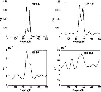
FIGURE 5.4 Power spectra obtained using the AR Yule-Walker method with a 15th-order model. The waveform consisted of two sinusoids at 240 and 280 Hz with various levels of noise. At the lowest noise levels, the two sinusoids are clearly distinguished, but appear to merge into one at the higher noise levels.

%Generate two closely space sine waves in white noise x = sig_noise([240 280],noise(i),N);

[PS,f] = pyulear(data,order,N,fs);

text(200,max(PS),[’SNR: ’,num2str(noise(i)), ‘db’]); xlabel(’Frequency (Hz)’); ylabel(’PS ’);

end

The output of this Example is presented in Figure 5.4. Note that the sinusoids are clearly identified at the two lower noise levels, but appear to merge

Copyright 2004 by Marcel Dekker, Inc. All Rights Reserved.

together for the higher noise levels. At the highest noise level, only a single, broad peak can be observed at a frequency that is approximately the average of the two sine wave frequencies. The number of points used will also strongly influence the resolution of all spectral methods. This behavior is explored in the problems at the end of this chapter.

NON-PARAMETRIC EIGENANALYSIS

FREQUENCY ESTIMATION

Eigenanalysis spectral methods are promoted as having better resolution and better frequency estimation characteristics, especially at high noise levels.* They are particularly effective in identifying sinusoidal, exponential, or other narrowband processes in white noise as these methods can eliminate much of the noise contribution. However, if the noise is not white, but contains some spectral features (i.e., colored noise), performance can be degraded. The key feature of eigenvector approaches is to divide the information contained in the data waveform (or autocorrelation function) into two subspaces: a signal subspace and a noise subspace. The eigen-decomposition produces eigenvalues of decreasing order, and, most importantly, eigenvectors that are orthonormal. Since all the eigenvectors are orthonormal, if those eigenvectors that are deemed part of the noise subspace are eliminated, the influence of that noise is effectively eliminated. Functions can be computed based on either signal or noise subspace and can be plotted in the frequency domain. Such plots generally show sharp peaks where sinusoids or narrowband processes exist. Unlike parametric methods discussed above, these techniques are not considered true power spectral estimators, since they do not preserve signal power, nor can the autocorrelation sequence be reconstructed by applying the Fourier transform to these estimators. Better termed frequency estimators, they provide spectra in relative units.

The most problematic aspect of applying eigenvector spectral analysis is selecting the appropriate dimension of the signal (or noise) subspace. If the number of narrowband processes is known, then the signal subspace can be dimensioned on this basis; since each real sinusoid is the sum of two complex exponentials, the signal subspace dimension should be twice the number of sinusoids, or narrowband processes present. In some applications the signal subspace can be determined by the size of the eigenvalues; however, this method does not often work in practice, particularly with short data segments† [Marple,

*Another application of eigen-decomposition, principal component analysis, will be presented in Chapter 9.

†A similar use of eigenvalues is the determination of dimension in multivariate data as shown in Chapter 9. The Scree plot, a plot of eigenvalue against eigenvalue numbers is sometime used to estimate signal subspace dimension (see Figure 9.7). This plot is also found in Example 5.3.

Copyright 2004 by Marcel Dekker, Inc. All Rights Reserved.

1987]. As with the determination of the order of an AR model, the determination of the signal subspace often relies the on trial-and-error approach.

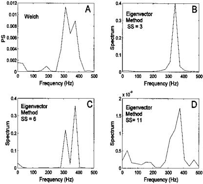
Figure 5.5 shows the importance of subspace dimension and illustrates both the strength and weaknesses of eigenvector spectral analysis. All four spectra were obtained from the same small data set (N = 32) consisting of two closely spaced sinusoids (320 and 380 Hz) in white noise (SNR = -7 db). Figure 5.5A shows the spectrum obtained using the classical, FFT-based Welch method. The other three plots show spectra obtained using eigenvector analysis, but with different partitions between the signal and noise subspaces. In Figure 5.5B, the spectrum was obtained using a signal subspace dimension of three. In this case, the size of the signal subspace is not large enough to differentiate

FIGURE 5.5 Spectra produced from a short data sequence (N = 32) containing two closely spaced sinusoids (320 and 380 Hz) in white noise (SNR = 7 db). The upper-left plot was obtained using the classical Welch method while the other three use eigenvector analysis with different partitions between the signal and noise subspace.

Copyright 2004 by Marcel Dekker, Inc. All Rights Reserved.

between the two closely spaced sinusoids, and, indeed, only a single peak is shown. When the signal subspace dimension is increased to 6 (Figure 5.5C) the two sinusoidal peaks are clearly distinguished and show better separation than with the classical method. However, when the signal subspace is enlarged further to a dimension of 11 (Figure 5.5D), the resulting spectrum contains small spurious peaks, and the two closely spaced sinusoids can no longer be distinguished. Hence, a signal subspace that is too large can be even more detrimental than one that is too small.

MATLAB Implementation

Two popular versions of frequency estimation based on eigenanalysis are the Pisarenko harmonic decomposition (PHP) and the MUltiple SIgnal Classifications (MUSIC) algorithms. These two eigenvector spectral analysis methods are available in the MATLAB Signal Processing Toolbox. Both methods have the same calling structure, a structure similar to that used by the AR routines. The command to evoke MUSIC algorithm is:

[PS, f,v,e] = pmusic(x, [p thresh], nfft, Fs, window, noverlap);

The last four input arguments are optional and have the same meaning as in pwelch, except that if window is a scalar or omitted, a rectangular window is used (as opposed to a Hamming window). The second argument is used to control the dimension of the signal (or noise) subspace. Since this parameter is critical to the successful application of the eigenvector approach, extra flexibility is provided. This argument can be either a scalar or vector. If only a single number is used, it will be taken as p, the dimension of the signal subspace. If the optional thresh is included, then eigenvalues below thresh times the minimum eigenvalue (i.e., thresh × λmin) will be assigned to the noise subspace; however, p still specifies the maximum signal subspace. Thus, thresh can be used to reduce the signal subspace dimension below that specified by p. To be meaningful, thresh must be > 1, otherwise the noise threshold would be < λmin and its subspace dimension would be 0 (hence, if thresh < 1 it is ignored). Similarly p must be < n, the dimension of the eigenvectors. The dimension of the eigenvectors, n, is either nfft, or if not specified, the default value of 256. Alternatively, n is the size of the data matrix if the corr option is used, and the input is the correlation matrix as described below.

As suggested above, the data argument, x, is also more flexible. If x is a vector, then it is taken as one observation of the signal as in previous AR and Welch routines. However, x can also be a matrix in which case the routine assumes that each row of x is a separate observation of the signal. For example, each row could be the output of an array of sensors or a single response in a

Copyright 2004 by Marcel Dekker, Inc. All Rights Reserved.

response ensemble. Such data are termed multivariate and are discussed in Chapter 9. Finally, the input argument x could be the correlation matrix. In this case, x must be a square matrix and the argument ‘corr’ should be added to the input sequence anywhere after the argument p. If the input is the correlation matrix, then the arguments window and noverlap have no meaning and are ignored.

The only required output argument is PS, which contains the power spectrum (more appropriately termed the pseudospectrum due to the limitation described previously). The second output argument, f, is the familiar frequency vector useful in plotting. The output argument, v, following f, is a matrix of eigenvectors spanning the noise subspace (one per column) and the final output argument, e, is either a vector of singular values (squared) or a vector of eigenvalues of the correlation matrix when the input argument ‘corr’ is used. An example of the use of the pmusic routine is given in the example below. An alternative eigenvector method can be implemented using the call peig. This routine has a calling structure identical to that of pmusic.

Example 5.3 This example compares classical, autoregressive and eigenanalysis spectral analysis methods, plots the singular values, generates Fig- ure 5.6, and uses an optimum value for AR model order and eigenanalysis subspace dimension.

%Example 5.3 and Figure 5.6

%Compares FFT-based, AR, and eigenanalysis spectral methods

close all; clear all;

%

%Generate a spectra of sinusoids and noise [data,t] = sig_noise([50 80 240 400],-10,N);

%Estimate the Welch spectrum for comparison, no window and

%no overlap

[PS,f] = pwelch(x,N,[],[],fs);

.......axis, labels, title.......

% Calculate the modified covariance spectrum for comparison

.......labels, title.......

% Generate the eigenvector spectrum using the MUSIC method

Copyright 2004 by Marcel Dekker, Inc. All Rights Reserved.

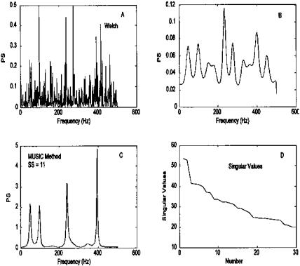
FIGURE 5.6 Spectrum obtained using 3 different methods applied to a waveform containing 4 equal amplitude sinusoids at frequencies of 50, 80, 240, and 400 Hz and white noise (SNR = -10 db; N = 1024). The eigenvector method (C) most clearly identifies the four components. The singular values determined from the eigenvalues (D) show a possible break or change in slope around n = 4 and another at n = 9, the latter being close to the actual signal subspace of 8.

%Get the singular values from the eigenvector routine

%and plot. Use high subspace dimension to get many singular

%values

subplot(2,2,4);

Copyright 2004 by Marcel Dekker, Inc. All Rights Reserved.

The plots produced by Example 5.3 are shown in Figure 5.6, and the strength of the eigenvector method for this task is apparent. In this example, the data length was quite long (N = 1024), but the SNR was low (-10 db). The signal consists of four equal amplitude sinusoids, two of which are closely spaced (50 and 80 Hz). While the spectrum produced by the classical Welch method does detect the four peaks, it also shows a number of other peaks in response to the noise. It would be difficult to determine, definitively and uniquely, the signal peaks from this spectrum. The AR method also detects the four peaks and greatly smooths the noise, but like the Welch method it shows spurious peaks related to the noise, and the rounded spectral shapes make it difficult to accurately determine the frequencies of the peaks. The eigenvector method not only resolves the four peaks, but provides excellent frequency resolution.

Figure 5.6 also shows a plot of the singular values as determined by pmusic. This plot can be used to estimate the dimensionality of multivariate data as detailed in Chapter 9. Briefly, the curve is examined for a break point between a steep and gentle slope, and this break point is taken as the dimensionality of the signal subspace. The idea is that a rapid decrease in the singular values is associated with the signal while a slower decrease indicates that the singular values are associated with the noise. Indeed, a slight break is seen around 9, approximately the correct value of the signal subspace. Unfortunately, welldefined break points are not always found when real data are involved.

The eigenvector method also performs well with short data sets. The behavior of the eigenvector method with short data sets and other conditions is explored in the problems.

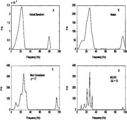
Most of the examples provided evaluate the ability of the various spectral methods to identify sinusoids or narrowband processes in the presence of noise, but what of a more complex spectrum? Example 5.4 explores the ability of the classical (FFT), model-based, and eigenvalue methods in estimating a more complicated spectrum. In this example, we use a linear process (one of the filters described in Chapter 4) driven by white noise to create a complicated broadband spectrum. Since the filter is driven by white noise, the spectrum of its output waveform should be approximately the same as the transfer function of the filter itself. The various spectral analysis techniques are applied to this waveform and their ability to estimate the actual filter Transfer Function is evaluated. The derivative FIR filter of Example 4.6 will be used, and its transfer function will be evaluated directly from the filter coefficients using the FFT.

Copyright 2004 by Marcel Dekker, Inc. All Rights Reserved.

Example 5.4 This example is designed to compare the ability of several spectral analysis approaches, classical, model-based, and eigenvalue, to estimate a complex, broadband spectrum. The filter is the same as that used in Example

4.6except that the derivative cutoff frequency has been increased to 0.25 fs/2.

%Example 5.4 and Figure 5.7

%Construct a spectrum for white noise passed through

%a FIR derivative filter. Use the filter in Example 4.6.

%Compare classical, model-based, and eigenvector methods

FIGURE 5.7 Estimation of a complex, broader-band spectrum using classical, model-based, and eigenvalue methods. (A) Transfer function of filter used to generate the data plotted a magnitude squared. (B) Estimation of the data spectrum using the Welch (FFT) method with 2 averages and maximum overlap. (C) Estimation of data spectrum using AR model, p = 17. (D) Estimation of data spectrum using an eigenvalue method with a subspace dimension of 13.

Copyright 2004 by Marcel Dekker, Inc. All Rights Reserved.

plot(f,PS,’k’);

.......labels and text.......

%

[PS,f] = music(x,13,N,fs);

subplot(2,2,4); % Eigenvector method (Music)

plot(f,PS,’k’);

.......labels and text.......

The plots produced by this program are shown in Figure 5.7. In Figure 5.7A, the filter’s transfer function is plotted as the magnitude squared so that it can be directly compared with the various spectral techniques that estimate the

Copyright 2004 by Marcel Dekker, Inc. All Rights Reserved.