Biosignal and Biomedical Image Processing MATLAB based Applications - John L. Semmlow

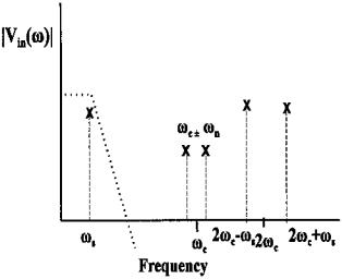
The spectrum of V ′(t) is shown in Figure 8.13. Note that the phase angle, θ, would have an influence on the magnitude of the signal, but not its frequency.

After lowpass digital filtering the higher frequency terms, ωct ± ωs will be reduced to near zero, so the output, Vout(t), becomes:

Since cos θ is a constant, the output of the phase sensitive detector is the demodulated signal, A(t), multiplied by this constant. The term phase sensitive is derived from the fact that the constant is a function of the phase difference, θ, between Vc(t) and Vin(t). Note that while θ is generally constant, any shift in phase between the two signals will induce a change in the output signal level, so this approach could also be used to detect phase changes between signals of constant amplitude.

The multiplier operation is similar to the sampling process in that it generates additional frequency components. This will reduce the influence of low frequency noise since it will be shifted up to near the carrier frequency. For example, consider the effect of the multiplier on 60 Hz noise (or almost any noise that is not near to the carrier frequency). Using the principle of superposition, only the noise component needs to be considered. For a noise component at frequency, ωn (Vin(t)NOISE = Vn cos (ωnt)). After multiplication the contribution at V ′(t) will be:

FIGURE 8.13 Frequency spectrum of the signal created by multiplying the Vin(t) by the carrier frequency. After lowpass filtering, only the original low frequency signal at ωs will remain.

Copyright 2004 by Marcel Dekker, Inc. All Rights Reserved.

and the new, complete spectrum for V ′(t) is shown in Figure 8.14.

The only frequencies that will not be attenuated in the input signal, Vin(t), are those around the carrier frequency that also fall within the bandwidth of the lowpass filter. Another way to analyze the noise attenuation characteristics of phase sensitive detection is to view the effect of the multiplier as shifting the lowpass filter’s spectrum to be symmetrical about the carrier frequency, giving it the form of a narrow bandpass filter (Figure 8.15). Not only can extremely narrowband bandpass filters be created this way (simply by having a low cutoff frequency in the lowpass filter), but more importantly the center frequency of the effective bandpass filter tracks any changes in the carrier frequency. It is these two features, narrowband filtering and tracking, that give phase sensitive detection its signal processing power.

MATLAB Implementation

Phase sensitive detection is implemented in MATLAB using simple multiplication and filtering. The application of a phase sensitive detector is given in Exam-

FIGURE 8.14 Frequency spectrum of the signal created by multiplying Vin(t) including low frequency noise by the carrier frequency. The low frequency noise is shifted up to ± the carrier frequency. After lowpass filtering, both the noise and higher frequency signal are greatly attenuated, again leaving only the original low frequency signal at ωs remaining.

Copyright 2004 by Marcel Dekker, Inc. All Rights Reserved.

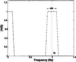
FIGURE 8.15 Frequency characteristics of a phase sensitive detector. The frequency response of the lowpass filter (solid line) is effectively “reflected” about the carrier frequency, fc, producing the effect of a narrowband bandpass filter (dashed line). In a phase sensitive detector the center frequency of this virtual bandpass filter tracks the carrier frequency.

ple 8.6 below. A carrier sinusoid of 250 Hz is modulated with a sawtooth wave with a frequency of 5 Hz. The AM signal is buried in noise that is 3.16 times the signal (i.e., SNR = -10 db).

Example 8.6 Phase Sensitive Detector. This example uses a phase sensitive detection to demodulate the AM signal and recover the signal from noise. The filter is chosen as a second-order Butterworth lowpass filter with a cutoff frequency set for best noise rejection while still providing reasonable fidelity to the sawtooth waveform. The example uses a sampling frequency of 2 kHz.

%Example 8.6 and Figure 8.16 Phase Sensitive Detection

%Set constants

%

Copyright 2004 by Marcel Dekker, Inc. All Rights Reserved.

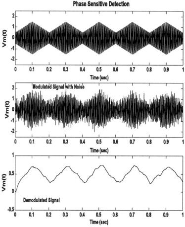
FIGURE 8.16 Application of phase sensitive detection to an amplitude-modulated signal. The AM signal consisted of a 250 Hz carrier modulated by a 5 Hz sawtooth (upper graph). The AM signal is mixed with white noise (SNR = −10db, middle graph). The recovered signal shows a reduction in the noise (lower graph).

Copyright 2004 by Marcel Dekker, Inc. All Rights Reserved.

%Add noise with 3.16 times power (10 db) of signal for SNR of

%-10 db

The lowpass filter was set to a cutoff frequency of 20 Hz (0.02 * fs/2) as a compromise between good noise reduction and fidelity. (The fidelity can be roughly assessed by the sharpness of the peaks of the recovered sawtooth wave.) A major limitation in this process were the characteristics of the lowpass filter: digital filters do not perform well at low frequencies. The results are shown in Figure 8.16 and show reasonable recovery of the demodulated signal from the noise.

Even better performance can be obtained if the interference signal is narrowband such as 60 Hz interference. An example of using phase sensitive detection in the presence of a strong 60 Hz signal is given in Problem 6 below.

PROBLEMS

1. Apply the Wiener-Hopf approach to a signal plus noise waveform similar to that used in Example 8.1, except use two sinusoids at 10 and 20 Hz in 8 db noise. Recall, the function sig_noise provides the noiseless signal as the third output to be used as the desired signal. Apply this optimal filter for filter lengths of 256 and 512.

Copyright 2004 by Marcel Dekker, Inc. All Rights Reserved.

2. Use the LMS adaptive filter approach to determine the FIR equivalent to the linear process described by the digital transfer function:

As with Example 8.2, plot the magnitude digital transfer function of the “unknown” system, H(z), and of the FIR “matching” system. Find the transfer function of the IIR process by taking the square of the magnitude of fft(b,n)./fft(a,n) (or use freqz). Use the MATLAB function filtfilt to produce the output of the IIR process. This routine produces no time delay between the input and filtered output. Determine the approximate minimum number of filter coefficients required to accurately represent the function above by limiting the coefficients to different lengths.

3.Generate a 20 Hz interference signal in noise with and SNR + 8 db; that is,

the interference signal is 8 db stronger that the noise. (Use sig_noise with an SNR of +8. ) In this problem the noise will be considered as the desired signal. Design an adaptive interference filter to remove the 20 Hz “noise.” Use an FIR filter with 128 coefficients.

4.Apply the ALE filter described in Example 8.3 to a signal consisting of two sinusoids of 10 and 20 Hz that are present simultaneously, rather that sequentially as in Example 8.3. Use a FIR filter lengths of 128 and 256 points. Evaluate the influence of modifying the delay between 4 and 18 samples.

5.Modify the code in Example 8.5 so that the reference signal is correlated with, but not the same as, the interference data. This should be done by convolving the reference signal with a lowpass filter consisting of 3 equal weights;

i.e:

b = [ 0.333 0.333 0.333].

For this more realistic scenario, note the degradation in performance as compared to Example 8.5 where the reference signal was identical to the noise.

6.Redo the phase sensitive detector in Example 8.6, but replace the white noise with a 60 Hz interference signal. The 60 Hz interference signal should have an amplitude that is 10 times that of the AM signal.

Copyright 2004 by Marcel Dekker, Inc. All Rights Reserved.

9

Multivariate Analyses:

Principal Component Analysis

and Independent Component Analysis

INTRODUCTION

Principal component analysis and independent component analysis fall within a branch of statistics known as multivariate analysis. As the name implies, multivariate analysis is concerned with the analysis of multiple variables (or measurements), but treats them as a single entity (for example, variables from multiple measurements made on the same process or system). In multivariate analysis, these multiple variables are often represented as a single vector variable that includes the different variables:

The ‘T’ stands for transposed and represents the matrix operation of switching rows and columns.* In this case, x is composed of M variables, each containing N (t = 1, . . . ,N ) observations. In signal processing, the observations are time samples, while in image processing they are pixels. Multivariate data, as represented by x above can also be considered to reside in M-dimensional space, where each spatial dimension contains one signal (or image).

In general, multivariate analysis seeks to produce results that take into

*Normally, all vectors including these multivariate variables are taken as column vectors, but to save space in this text, they are often written as row vectors with the transpose symbol to indicate that they are actually column vectors.

Copyright 2004 by Marcel Dekker, Inc. All Rights Reserved.

account the relationship between the multiple variables as well as within the variables, and uses tools that operate on all of the data. For example, the covariance matrix described in Chapter 2 (Eq. (19), Chapter 2, and repeated in Eq.

(4) below) is an example of a multivariate analysis technique as it includes information about the relationship between variables (their covariance) and information about the individual variables (their variance). Because the covariance matrix contains information on both the variance within the variables and the covariance between the variables, it is occasionally referred to as the variance– covariance matrix.

A major concern of multivariate analysis is to find transformations of the multivariate data that make the data set smaller or easier to understand. For example, is it possible that the relevant information contained in a multidimensional variable could be expressed using fewer dimensions (i.e., variables) and might the reduced set of variables be more meaningful than the original data set? If the latter were true, we would say that the more meaningful variables were hidden, or latent, in the original data; perhaps the new variables better represent the underlying processes that produced the original data set. A biomedical example is found in EEG analysis where a large number of signals are acquired above the region of the cortex, yet these multiple signals are the result of a smaller number of neural sources. It is the signals generated by the neural sources—not the EEG signals per se—that are of interest.

In transformations that reduce the dimensionality of a multi-variable data set, the idea is to transform one set of variables into a new set where some of the new variables have values that are quite small compared to the others. Since the values of these variables are relatively small, they must not contribute very much information to the overall data set and, hence, can be eliminated.* With the appropriate transformation, it is sometimes possible to eliminate a large number of variables that contribute only marginally to the total information.

The data transformation used to produce the new set of variables is often a linear function since linear transformations are easier to compute and their results are easier to interpret. A linear transformation can be represent mathematically as:

where wij is a constant coefficient that defines the transformation.

*Evaluating the significant of a variable by the range of its values assumes that all the original variables have approximately the same range. If not, some form of normalization should be applied to the original data set.

Copyright 2004 by Marcel Dekker, Inc. All Rights Reserved.

Since this transformation is a series of equations, it can be equivalently

yM(t) xM(t)

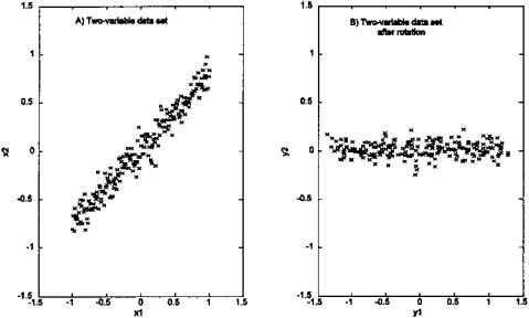
As a linear transformation, this operation can be interpreted as a rotation and possibly scaling of the original data set in M-dimensional space. An example of how a rotation of a data set can produce a new data set with fewer major variables is shown in Figure 9.1 for a simple two-dimensional (i.e., two variable) data set. The original data set is shown as a plot of one variable against the other, a so-called scatter plot, in Figure 9.1A. The variance of variable x1 is 0.34 and the variance of x2 is 0.20. After rotation the two new variables, y1 and y2 have variances of 0.53 and 0.005, respectively. This suggests that one variable, y1, contains most of the information in the original two-variable set. The

FIGURE 9.1 A data set consisting of two variables before (left graph) and after (right graph) linear rotation. The rotated data set still has two variables, but the variance on one of the variables is quite small compared to the other.

Copyright 2004 by Marcel Dekker, Inc. All Rights Reserved.

goal of this approach to data reduction is to find a matrix W that will produce such a transformation.

The two multivariate techniques discussed below, principal component analysis and independent component analysis, differ in their goals and in the criteria applied to the transformation. In principal component analysis, the object is to transform the data set so as to produce a new set of variables (termed principal components) that are uncorrelated. The goal is to reduce the dimensionality of the data, not necessarily to produce more meaningful variables. We will see that this can be done simply by rotating the data in M-dimensional space. In independent component analysis, the goal is a bit more ambitious: to find new variables (components) that are both statistically independent and nongaussian.

PRINCIPAL COMPONENT ANALYSIS

Principal component analysis (PCA) is often referred to as a technique for reducing the number of variables in a data set without loss of information, and as a possible process for identifying new variables with greater meaning. Unfortunately, while PCA can be, and is, used to transform one set of variables into another smaller set, the newly created variables are not usually easy to interpret. PCA has been most successful in applications such as image compression where data reduction—and not interpretation—is of primary importance. In many applications, PCA is used only to provide information on the true dimensionality of a data set. That is, if a data set includes M variables, do we really need all M variables to represent the information, or can the variables be recombined into a smaller number that still contain most of the essential information (Johnson, 1983)? If so, what is the most appropriate dimension of the new data set?

PCA operates by transforming a set of correlated variables into a new set of uncorrelated variables that are called the principal components. Note that if the variables in a data set are already uncorrelated, PCA is of no value. In addition to being uncorrelated, the principal components are orthogonal and are ordered in terms of the variability they represent. That is, the first principle component represents, for a single dimension (i.e., variable), the greatest amount of variability in the original data set. Each succeeding orthogonal component accounts for as much of the remaining variability as possible.

The operation performed by PCA can be described in a number of ways, but a geometrical interpretation is the most straightforward. While PCA is applicable to data sets containing any number of variables, it is easier to describe using only two variables since this leads to readily visualized graphs. Figure 9.2A shows two waveforms: a two-variable data set where each variable is a different mixture of the same two sinusoids added with different scaling factors. A small amount of noise was also added to each waveform (see Example 9.1).

Copyright 2004 by Marcel Dekker, Inc. All Rights Reserved.