Biosignal and Biomedical Image Processing MATLAB based Applications - John L. Semmlow

FIGURE 6.15 The Rihaczek-Margenau distribution to a chirp signal. Note that this distribution shows the most constant amplitude throughout the time-fre- quency plot, but does show some small cross products that diagonal away from the side. In addition, the frequency peak is not as well-defined as in the other distributions.

distributions. Assume a sample frequency of 300 Hz and a 2 sec time period. Use analytical signal.

6.Repeat Problem 5 above using a chirp signal that varies between 20 and

100Hz, with the same amplitude of added noise.

7.Repeat Problem 6 with twice the amount of added noise.

8.Repeat Problems 6 and 7 using the Rihaczek-Margenau distribution.

Copyright 2004 by Marcel Dekker, Inc. All Rights Reserved.

7

Wavelet Analysis

INTRODUCTION

Before introducing the wavelet transform we review some of the concepts regarding transforms presented in Chapter 2. A transform can be thought of as a remapping of a signal that provides more information than the original. The Fourier transform fits this definition quite well because the frequency information it provides often leads to new insights about the original signal. However, the inability of the Fourier transform to describe both time and frequency characteristics of the waveform led to a number of different approaches described in the last chapter. None of these approaches was able to completely solve the time–frequency problem. The wavelet transform can be used as yet another way to describe the properties of a waveform that changes over time, but in this case the waveform is divided not into sections of time, but segments of scale.

In the Fourier transform, the waveform was compared to a sine func- tion—in fact, a whole family of sine functions at harmonically related frequencies. This comparison was carried out by multiplying the waveform with the sinusoidal functions, then averaging (using either integration in the continuous domain, or summation in the discrete domain):

Eq. (1) is the continuous form of Eq. (6) in Chapter 3 used to define the discrete Fourier transform. As discussed in Chapter 2, almost any family of func-

Copyright 2004 by Marcel Dekker, Inc. All Rights Reserved.

tions could be used to probe the characteristics of a waveform, but sinusoidal functions are particularly popular because of their unique frequency characteristics: they contain energy at only one specific frequency. Naturally, this feature makes them ideal for probing the frequency makeup of a waveform, i.e., its frequency spectrum.

Other probing functions can be used, functions chosen to evaluate some particular behavior or characteristic of the waveform. If the probing function is of finite duration, it would be appropriate to translate, or slide, the function over the waveform, x(t), as is done in convolution and the short-term Fourier transform (STFT), Chapter 6’s Eq. (1), repeated here:

where f, the frequency, also serves as an indication of family member, and w(t − τ) is some sliding window function where t acts to translate the window over x. More generally, a translated probing function can be written as:

where f(t)m is some family of functions, with m specifying the family number. This equation was presented in discrete form in Eq. (10), Chapter 2.

If the family of functions, f(t)m, is sufficiently large, then it should be able to represent all aspects the waveform x(t). This would then allow x(t) to be reconstructed from X(t,m) making this transform bilateral as defined in Chapter 2. Often the family of basis functions is so large that X(t,m) forms a redundant set of descriptions, more than sufficient to recover x(t). This redundancy can sometimes be useful, serving to reduce noise or acting as a control, but may be simply unnecessary. Note that while the Fourier transform is not redundant, most transforms represented by Eq. (3) (including the STFT and all the distributions in Chapter 6) would be, since they map a variable of one dimension (t) into a variable of two dimensions (t,m).

THE CONTINUOUS WAVELET TRANSFORM

The wavelet transform introduces an intriguing twist to the basic concept defined by Eq. (3). In wavelet analysis, a variety of different probing functions may be used, but the family always consists of enlarged or compressed versions of the basic function, as well as translations. This concept leads to the defining equation for the continuous wavelet transform (CWT):

Copyright 2004 by Marcel Dekker, Inc. All Rights Reserved.

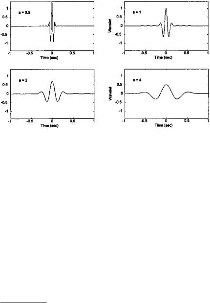
FIGURE 7.1 A mother wavelet (a = 1) with two dilations (a = 2 and 4) and one contraction (a = 0.5).

where b acts to translate the function across x(t) just as t does in the equations above, and the variable a acts to vary the time scale of the probing function, ψ. If a is greater than one, the wavelet function, ψ, is stretched along the time axis, and if it is less than one (but still positive) it contacts the function. Negative values of a simply flip the probing function on the time axis. While the probing function ψ could be any of a number of different functions, it always takes on an oscillatory form, hence the term “wavelet.” The * indicates the operation of complex conjugation, and the normalizing factor l/√a ensures that the energy is the same for all values of a (all values of b as well, since translations do not alter wavelet energy). If b = 0, and a = 1, then the wavelet is in its natural form, which is termed the mother wavelet;* that is, ψ1,o(t) ≡ ψ(t). A mother wavelet is shown in Figure 7.1 along with some of its family members produced by dilation and contraction. The wavelet shown is the popular Morlet wavelet, named after a pioneer of wavelet analysis, and is defined by the equation:

*Individual members of the wavelet family are specified by the subscripts a and b; i.e., ψa,b. The mother wavelet, ψ1,0, should not to be confused with the mother of all Wavelets which has yet to be discovered.

Copyright 2004 by Marcel Dekker, Inc. All Rights Reserved.

The wavelet coefficients, W(a,b), describe the correlation between the waveform and the wavelet at various translations and scales: the similarity between the waveform and the wavelet at a given combination of scale and position, a,b. Stated another way, the coefficients provide the amplitudes of a series of wavelets, over a range of scales and translations, that would need to be added together to reconstruct the original signal. From this perspective, wavelet analysis can be thought of as a search over the waveform of interest for activity that most clearly approximates the shape of the wavelet. This search is carried out over a range of wavelet sizes: the time span of the wavelet varies although its shape remains the same. Since the net area of a wavelet is always zero by design, a waveform that is constant over the length of the wavelet would give rise to zero coefficients. Wavelet coefficients respond to changes in the waveform, more strongly to changes on the same scale as the wavelet, and most strongly, to changes that resemble the wavelet. Although a redundant transformation, it is often easier to analyze or recognize patterns using the CWT. An example of the application of the CWT to analyze a waveform is given in the section on MATLAB implementation.

If the wavelet function, ψ(t), is appropriately chosen, then it is possible to reconstruct the original waveform from the wavelet coefficients just as in the Fourier transform. Since the CWT decomposes the waveform into coefficients of two variables, a and b, a double summation (or integration) is required to recover the original signal from the coefficients:

and 0 < C < ∞ (the so-called admissibility condition) for recovery using Eq.

(6).

In fact, reconstruction of the original waveform is rarely performed using the CWT coefficients because of the redundancy in the transform. When recovery of the original waveform is desired, the more parsimonious discrete wavelet transform is used, as described later in this chapter.

Wavelet Time–Frequency Characteristics

Wavelets such as that shown in Figure 7.1 do not exist at a specific time or a specific frequency. In fact, wavelets provide a compromise in the battle between time and frequency localization: they are well localized in both time and fre-

Copyright 2004 by Marcel Dekker, Inc. All Rights Reserved.

quency, but not precisely localized in either. A measure of the time range of a specific wavelet, ∆tψ, can be specified by the square root of the second moment of a given wavelet about its time center (i.e., its first moment) (Akansu & Haddad, 1992):

∞

∫ (t − t0)2*ψ(t/a)*2dt

where t0 is the center time, or first moment of the wavelet, and is given by:

∞

∫ t*ψ(t/a)*2dt

∫ *ψ(t/a)*2dt

−∞

Similarly the frequency range, ∆ωψ, is given by:

∞

∫ (ω − ω0)2*Ψ(ω)*2dω

where Ψ(ω) is the frequency domain representation (i.e., Fourier transform) of ψ(t/a), and ω0 is the center frequency of Ψ(ω). The center frequency is given by an equation similar to Eq. (8):

∞

∫ ω*Ψ(ω)*2dω

∫ *Ψ(ω)*2dω

−∞

The time and frequency ranges of a given family can be obtained from the mother wavelet using Eqs. (7) and (9). Dilation by the variable a changes the time range simply by multiplying ∆tψ by a. Accordingly, the time range of ψa,0 is defined as ∆tψ(a) = *a*∆tψ. The inverse relationship between time and frequency is shown in Figure 7.2, which was obtained by applying Eqs. (7–10) to the Mexican hat wavelet. (The code for this is given in Example 7.2.) The Mexican hat wavelet is given by the equation:

Copyright 2004 by Marcel Dekker, Inc. All Rights Reserved.

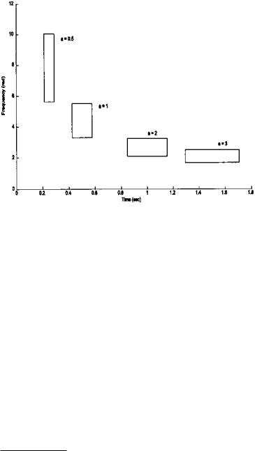
FIGURE 7.2 Time–frequency boundaries of the Mexican hat wavelet for various values of a. The area of each of these boxes is constant (Eq. (12)). The code that generates this figure is based on Eqs. (7–10) and is given in Example 7.2.

The frequency range, or bandwidth, would be the range of the mother Wavelet divided by a: ∆ωψ(a) = ∆ωψ /*a*. If we multiply the frequency range by the time range, the a’s cancel and we are left with a constant that is the product of the constants produced by Eq. (7) and (9):

Eq. (12) shows that the product of the ranges is invariant to dilation* and that the ranges are inversely related; increasing the frequency range, ∆ωψ(a), decreases the time range, ∆tψ(a). These ranges correlate to the time and frequency resolution of the CWT. Just as in the short-term Fourier transform, there is a time–frequency trade-off (recall Eq. (3) in Chapter 6): decreasing the wavelet time range (by decreasing a) provides a more accurate assessment of time characteristics (i.e., the ability to separate out close events in time) at the expense of frequency resolution, and vice versa.

*Translations (changes in the variable b), do alter either the time or frequency resolution; hence, both time and frequency resolution, as well as their product, are independent of the value of b.

Copyright 2004 by Marcel Dekker, Inc. All Rights Reserved.

Since the time and frequency resolutions are inversely related, the CWT will provide better frequency resolution when a is large and the length of the wavelet (and its effective time window) is long. Conversely, when a is small, the wavelet is short and the time resolution is maximum, but the wavelet only responds to high frequency components. Since a is variable, there is a built-in trade-off between time and frequency resolution, which is key to the CWT and makes it well suited to analyzing signals with rapidly varying high frequency components superimposed on slowly varying low frequency components.

MATLAB Implementation

A number of software packages exist in MATLAB for computing the continuous wavelet transform, including MATLAB’s Wavelet Toolbox and Wavelab which is available free over the Internet: (www.stat.stanford.edu/ wavelab/). However, it is not difficult to implement Eq. (4) directly, as illustrated in the example below.

Example 7.1 Write a program to construct the CWT of a signal consisting of two sequential sine waves of 10 and 40 Hz. (i.e. the signal shown in Figure 6.1). Plot the wavelet coefficients as a function of a and b. Use the Morlet wavelet.

The signal waveform is constructed as in Example 6.1. A time vector, ti, is generated that will be used to produce the positive half of the wavelet. This vector is initially scaled so that the mother wavelet (a = 1) will be ± 10 sec long. With each iteration, the value of a is adjusted (128 different values are used in this program) and the wavelet time vector is it then scaled to produce the appropriate wavelet family member. During each iteration, the positive half of the Morlet wavelet is constructed using the defining equation (Eq. (5)), and the negative half is generated from the positive half by concatenating a time reversed (flipped) version with the positive side. The wavelet coefficients at a given value of a are obtained by convolution of the scaled wavelet with the signal. Since convolution in MATLAB produces extra points, these are removed symmetrically (see Chapter 2), and the coefficients are plotted three-dimension- ally against the values of a and b. The resulting plot, Figure 7.3, reflects the time–frequency characteristics of the signal which are quantitatively similar to those produced by the STFT and shown in Figure 6.2.

%Example 7.1 and Figure 7.3

%Generate 2 sinusoids that change frequency in a step-like

%manner

%Apply the continuous wavelet transform and plot results

clear all; close all;

%Set up constants

Copyright 2004 by Marcel Dekker, Inc. All Rights Reserved.

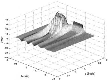
FIGURE 7.3 Wavelet coefficients obtained by applying the CWT to a waveform consisting of two sequential sine waves of 10 and 40 Hz, as shown in Figure 6.1. The Morlet wavelet was used.

Copyright 2004 by Marcel Dekker, Inc. All Rights Reserved.

%Calculate continuous Wavelet transform

%Morlet wavelet, Eq. (5)

% Plot in 3 dimensions d = fliplr(CW_Trans); mesh(a,b,CW_Trans);

***** labels and view angle *****

In this example, a was modified by division with a linearly increasing value. Often, wavelet scale is modified based on octaves or fractions of octaves.

A determination of the time–frequency boundaries of a wavelet though MATLAB implementation of Eqs. (7–10) is provided in the next example.

Example 7.2 Find the time–frequency boundaries of the Mexican hat wavelet.

For each of 4 values of a, the scaled wavelet is constructed using an approach similar to that found in Example 7.1. The magnitude squared of the frequency response is calculated using the FFT. The center time, t0, and center frequency, w0, are constructed by direct application of Eqs. (8) and (10). Note that since the wavelet is constructed symmetrically about t = 0, the center time, t0, will always be zero, and an appropriate offset time, t1, is added during plotting. The time and frequency boundaries are calculated using Eqs. (7) and (9), and the resulting boundaries as are plotted as a rectangle about the appropriate time and frequency centers.

%Example 7.2 and Figure 7.2

%Plot of wavelet boundaries for various values of ’a’

%Determines the time and scale range of the Mexican wavelet.

%Uses the equations for center time and frequency and for time

%and frequency spread given in Eqs. (7–10)

%

Copyright 2004 by Marcel Dekker, Inc. All Rights Reserved.