Biosignal and Biomedical Image Processing MATLAB based Applications - John L. Semmlow

FIGURE 9.8 Plot of the first two principal components and the original two sources. Note that the components are not the same as the original sources. Even thought they are uncorrelated (see covariance matrix on the next page), they cannot be independent since they are still mixtures of the two sources.

.......labels and title....................

%

% Calculate Eigenvalue ratio total_eigen = sum(eigen); for i = 1:5

pct(i) = sum(eigen(i:5))/total_eigen;

%

% Print Scaled Eigenvalues and Covariance Matrix of Principal

Copyright 2004 by Marcel Dekker, Inc. All Rights Reserved.

%Components S = cov(pc)

%Plot Principal Components and Original Data figure;

The five variables are plotted below in Figure 9.7. Note that the strong dependence between the variables (they are the product of only two different sources plus noise) is not entirely obvious from the time plots. The new covariance matrix taken from the principal components shows that all five components are uncorrelated, and also gives the variance of the five principal components

0.5708 −0.0000 0.0000 −0.0000 0.0000

−0.0000 0.0438 0.0000 −0.0000 0.0000 0.0000 0.0000 0.0297 −0.0000 0.0000

−0.0000 −0.0000 −0.0000 0.0008 0.0000

0.0000 0.0000 0.0000 0.0000 0.0008

The percentage of variance accounted by the sums of the various eigenvalues is given by the program as:

Note that the last three components account for only 4.84% of the variance of the data. This suggests that the actual dimension of the data is closer to two than to five. The scree plot, the plot of eigenvalue versus component number, provides another method for checking data dimensionality. As shown in Figure 9.6, there is a break in the slope at 2, again suggesting that the actual dimension of the data set is two (which we already know since it was created using only two independent sources).

The first two principal components are shown in Figure 9.8, along with the waveforms of the original sources. While the principal components are uncorrelated, as shown by the covariance matrix above, they do not reflect the two

Copyright 2004 by Marcel Dekker, Inc. All Rights Reserved.

independent data sources. Since they are still mixtures of the two sources they can not be independent even though they are uncorrelated. This occurs because the variables do not have a gaussian distribution, so that decorrelation does not imply independence. Another technique described in the next section can be used to make the variables independent, in which case the original sources can be recovered.

INDEPENDENT COMPONENT ANALYSIS

The application of principal component analysis described in Example 9.1 shows that decorrelating the data is not sufficient to produce independence between the variables, at least when the variables have nongaussian distributions. Independent component analysis seeks to transform the original data set into number of independent variables. The motivation for this transformation is primarily to uncover more meaningful variables, not to reduce the dimensions of the data set. When data set reduction is also desired it is usually accomplished by preprocessing the data set using PCA.

One of the more dramatic applications of independent component analysis (ICA) is found in the cocktail party problem. In this situation, multiple people are speaking simultaneously within the same room. Assume that their voices are recorded from a number of microphones placed around the room, where the number of microphones is greater than, or equal to, the number of speakers. Figure 9.9 shows this situation for two microphones and two speakers. Each microphone will pick up some mixture of all of the speakers in the room. Since presumably the speakers are generating signals that are independent (as would be the case in a real cocktail party), the successful application of independent component analysis to a data set consisting of microphone signals should recover the signals produced by the different speakers. Indeed, ICA has been quite successful in this problem. In this case, the goal is not to reduce the number of signals, but to produce signals that are more meaningful; specifically, the speech of the individual speakers. This problem is similar to the analysis of EEG signals where many signals are recorded from electrodes placed around the head, and these signals represent combinations of underlying neural sources.

The most significant computational difference between ICA and PCA is that PCA uses only second-order statistics (such as the variance which is a function of the data squared) while ICA uses higher-order statistics (such as functions of the data raised to the fourth power). Variables with a Gaussian distribution have zero statistical moments above second-order, but most signals do not have a Gaussian distribution and do have higher-order moments. These higher-order statistical properties are put to good use in ICA.

The basis of most ICA approaches is a generative model; that is, a model that describes how the measured signals are produced. The model assumes that

Copyright 2004 by Marcel Dekker, Inc. All Rights Reserved.

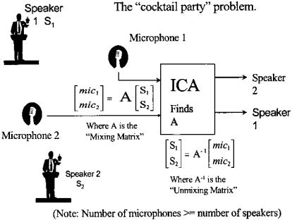
FIGURE 9.9 A schematic of the cocktail party problem where two speakers are talking simultaneously and their voices are recorded by two microphones. Each microphone detects the output of both speakers. The problem is to unscramble, or unmix, the two signals from the combinations in the microphone signals. No information is known about the content of the speeches nor the placement of the microphones and speakers.

the measured signals are the product of instantaneous linear combinations of the independent sources. Such a model can be stated mathematically as:

xi (t) = ai1 s1(t) + ai2 s2(t) + . . . + aiN sN (t) for i = 1, . . . , N (13)

Note that this is a series of equations for the N different signal variables, xi(t). In discussions of the ICA model equation, it is common to drop the time function. Indeed, most ICA approaches do not take into account the ordering of variable elements; hence, the fact that s and x are time functions is irrelevant.

xn(t) sn(t)

Copyright 2004 by Marcel Dekker, Inc. All Rights Reserved.

which can be written succinctly as:

where s is a vector composed of all the source signals,* A is the mixing matrix composed of the constant elements ai,j, and x is a vector of the measured signals. The model described by Eqs. (13) and (14) is also known as a latent variables model since the source variables, s, cannot be observed directly: they are hidden, or latent, in x. Of course the principle components in PCA are also latent variables; however, since they are not independent they are usually difficult to interpret. Note that noise is not explicitly stated in the model, although ICA methods will usually work in the presence of moderate noise (see Example 9.3). ICA techniques are used to solve for the mixing matrix, A, from which the independent components, s, can be obtained through simple matrix inversion:

If the mixing matrix is known or can be determined, then the underlying sources can be found simply by solving Eq. (16). However, ICA is used in the more general situation where the mixing matrix is not known. The basic idea is that if the measured signals, x, are related to the underlying source signals, s, by a linear transformation (i.e., a rotation and scaling operation) as indicated by Eqs. (14) and (15), then some inverse transformation (rotation/scaling) can be found that recovers the original signals. To estimate the mixing matrix, ICA needs to make only two assumptions: that the source variables, s, are truly independent;† and that they are non-Gaussian. Both conditions are usually met when the sources are real signals. A third restriction is that the mixing matrix must be square; in other words, the number of sources should equal the number of measured signals. This is not really a restriction since PCA can be always be applied to reduce the dimension of the data set, x, to equal that of the source data set, s.

The requirement that the underlying signals be non-Gaussian stems from the fact that ICA relies on higher-order statistics to separate the variables. Higher-order statistics (i.e., moments and related measures) of Gaussian signals are zero. ICA does not require that the distribution of the source variables be known, only that they not be Gaussian. Note that if the measured variables are already independent, ICA has nothing to contribute, just as PCA is of no use if the variables are already uncorrelated.

The only information ICA has available is the measured variables; it has no information on either the mixing matrix, A, or the underlying source vari-

*Note that the source signals themselves are also vectors. In this notation, the individual signals are considered as components of the single source vector, s.

†In fact, the requirement for strict independence can be relaxed somewhat in many situations.

Copyright 2004 by Marcel Dekker, Inc. All Rights Reserved.

ables, s. Hence, there are some limits to what ICA can do: there are some unresolvable ambiguities in the components estimated by ICA. Specifically, ICA cannot determine the variances, hence the energies or amplitudes, of the actual sources. This is understandable if one considers the cocktail party problem. The sounds from a loudmouth at the party could be offset by the positions and gains of the various microphones, making it impossible to identify definitively his excessive volume. Similarly a soft-spoken party-goer could be closer to a number of the microphones and appear unduly loud in the recorded signals. Unless something is known about the mixing matrix (in this case the position and gains of the microphones with respect to the various speakers), this ambiguity cannot be resolved. Since the amplitude of the signals cannot be resolved, it is usual to fix the amplitudes so that a signal’s variance is one. It is also impossible, for the same reasons, to determine the sign of the source signal, although this is not usually of much concern in most applications.

A second restriction is that, unlike PCA, the order of the components cannot be established. This follows from the arguments above: to establish the order of a given signal would require some information about the mixing matrix which, by definition, is unknown. Again, in most applications this is not a serious shortcoming.

The determination of the independent components begins by removing the mean values of the variables, also termed centering the data, as in PCA. The next step is to whiten the data, also know as sphering the data. Data that have been whitened are uncorrelated (as are the principal components), but, in addition, all of the variables have variances of one. PCA can be used for both these operations since it decorrelates the data and provides information on the variance of the decorrelated data in the form of the eigenvectors. Figure 9.10 shows the scatter plot of the data used in Figure 9.1 before and after whitening using PCA to decorrelate the data then scaling the components to have unit variances.

The independent components are determined by applying a linear transformation to the whitened data. Since the observations are a linear transformation of the underlying signals, s, (Eq. (15)) one should be able to be reconstruct them from a (inverse) linear transformation to the observed signals, x. That is, a given component could be obtained by the transformation:

where ic, the independent component, is an estimate of the original signal, and b is the appropriate vector to reconstruct that independent component. There are quite a number of different approaches for estimating b, but they all make use of an objective function that relates to variable independence. This function is maximized (or minimized) by an optimization algorithm. The various approaches differ in the specific objective function that is optimized and the optimization method that is used.

Copyright 2004 by Marcel Dekker, Inc. All Rights Reserved.

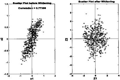
FIGURE 9.10 Two-variable multivariate data before (left) and after (right) whitening. Whitened data has been decorrelated and the resultant variables scaled so that their variance is one. Note that the whitened data has a generally circular shape. A whitened three-variable data set would have a spherical shape, hence the term sphering the data.

One of the most intuitive approaches uses an objective function that is related to the non-gaussianity of the data set. This approach takes advantage of the fact that mixtures tend to be more gaussian than the distribution of independent sources. This is a direct result of the central limit theorem which states that the sum of k independent, identically distributed random variables converges to a Gaussian distribution as k becomes large, regardless of the distribution of the individual variables. Hence, mixtures of non-Gaussian sources will be more Gaussian than the unmixed sources. This was demonstrated in Figure 2.1 using averages of uniformly distributed random data. Here we demonstrate the action of the central limit theorem using a deterministic function. In Figure 9.11A, a Gaussian distribution is estimated using the histogram of a 10,000-point sequence of Gaussian noise as produced by the MATLAB function randn. A distribution that is closely alined with an actual gaussian distribution (dotted line) is seen. A similarly estimated distribution of a single sine wave is shown in Figure 9.11B along with the Gaussian distribution. The sine wave distribution (solid line) is quite different from Gaussian (dashed line). However, a mixture of only two independent sinusoids (having different frequencies) is seen to be

Copyright 2004 by Marcel Dekker, Inc. All Rights Reserved.

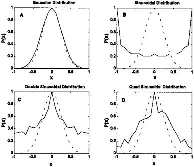
FIGURE 9.11 Approximate distributions for four variables determined from histograms of 10,0000-point waveforms. (A) Gaussian noise (from the MATLAB randn function). (B) Single sinusoid at 100 Hz. (C) Two sinusoids mixed together (100 and 30 Hz). (D) Four sinusoids mixed together (100, 70, 30, and 25 Hz). Note that larger mixtures produce distributions that look more like Gaussian distributions.

much closer to the Gaussian distribution (Figure 9.11C). The similarity improves as more independent sinusoids are mixed together, as seen in Figure 9.11D which shows the distribution obtained when four sinusoids (not harmonically related) are added together.

To take advantage of the relationship between non-gaussianity and component independence requires a method to measure gaussianity (or lack thereof). With such a measure, it would be possible to find b in Eq. (14) by adjusting b until the measured non-gaussianity of the transformed data set, ici, is maximum. One approach to quantifying non-gaussianity is to use kurtosis, the fourth-order cumulant of a variable, that is zero for Gaussian data and nonzero otherwise. Other approaches use an information-theoretic measure termed negentropy. Yet another set of approaches uses mutual information as the objective function to be minimized. An excellent treatment of the various approaches, their strengths

Copyright 2004 by Marcel Dekker, Inc. All Rights Reserved.

and weaknesses, can be found in Hyva¨rinen et al. (2001), as well as Cichicki et al. (2002).

MATLAB Implementation

Development of an ICA algorithm is not a trivial task; however, a number of excellent algorithms can be downloaded from the Internet in the form of MATLAB m-files. Two particularly useful algorithms are the FastICA algorithm developed by the ICA Group at Helsinki University:

http://www.cis.hut.fi/projects/ica/fastica/fp.html

and the Jade algorithm for real-valued signals developed by J.-F. Cardoso:

http://sig.enst.fr/ cardoso/stuff.html.

The Jade algorithm is used in the example below, although the FastICA algorithm allows greater flexibility, including an interactive mode.

Example 9.3 Construct a data set consisting of five observed signals that are linear combinations of three different waveforms. Apply PCA and plot the scree plot to determine the actual dimension of the data set. Apply the Jade ICA algorithm given the proper dimensions to recover the individual components.

%Example 9.3 and Figure 9.12, 9.13, 9.14, and 9.15

%Example of ICA

%Create a mixture using three different signals mixed five ways

%plus noise

%Use this in PCA and ICA analysis

.07*randn(1,N);

%

% Plot original signals displaced for viewing

Copyright 2004 by Marcel Dekker, Inc. All Rights Reserved.

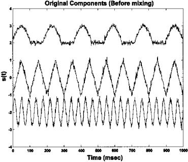
FIGURE 9.12 The three original source signals used to create the mixture seen in Figure 9.14 and used in Example 9.3.

plot(t,s1–2,’k’,t,s2,’k’,t,s3 2,’k’); xlabel(’Time (sec)’); ylabel(’s(t)’); title(’Original Components (Before mixing)’);

%

%Combine the 3 source signals 5 different ways. Define the mix-

%ing matrix

%

% Center data and plot mixed signals for i = 1:5

X(i,:) = X(i,:)—mean(X(i,:)); plot(t,X(i,:) 2*(i-1),’k’); hold on;

end

......labels and title..........

Copyright 2004 by Marcel Dekker, Inc. All Rights Reserved.