Biosignal and Biomedical Image Processing MATLAB based Applications - John L. Semmlow

or orthonormal:† the scalar product computations (or projections) can be done on each axes (i.e., on each family member) independently of the others.

CONVOLUTION, CORRELATION, AND COVARIANCE

Convolution, correlation, and covariance are similar-sounding terms and are similar in the way they are calculated. This similarity is somewhat misleading—at least in the case of convolution—since the areas of application and underlying concepts are not the same.

Convolution and the Impulse Response

Convolution is an important concept in linear systems theory, solving the need for a time domain operation equivalent to the Transfer Function. Recall that the Transfer Function is a frequency domain concept that is used to calculate the output of a linear system to any input. Convolution can be used to define a general input–output relationship in the time domain analogous to the Transfer Function in the frequency domain. Figure 2.6 demonstrates this application of convolution. The input, x(t), the output, y(t), and the function linking the two through convolution, h(t), are all functions of time; hence, convolution is a time domain operation. (Ironically, convolution algorithms are often implemented in the frequency domain to improve the speed of the calculation.)

The basic concept behind convolution is superposition. The first step is to determine a time function, h(t), that tells how the system responds to an infinitely short segment of the input waveform. If superposition holds, then the output can be determined by summing (integrating) all the response contributions calculated from the short segments. The way in which a linear system responds to an infinitely short segment of data can be determined simply by noting the system’s response to an infinitely short input, an infinitely short pulse. An infinitely short pulse (or one that is at least short compared to the dynamics of the system) is termed an impulse or delta function (commonly denoted δ(t)), and the response it produces is termed the impulse response, h(t).

FIGURE 2.6 Convolution as a linear process.

†Orthonormal vectors are orthogonal, but also have unit length.

Copyright 2004 by Marcel Dekker, Inc. All Rights Reserved.

Given that the impulse response describes the response of the system to an infinitely short segment of data, and any input can be viewed as an infinite string of such infinitesimal segments, the impulse response can be used to determine the output of the system to any input. The response produced by an infinitely small data segment is simply this impulse response scaled by the magnitude of that data segment. The contribution of each infinitely small segment can be summed, or integrated, to find the response created by all the segments.

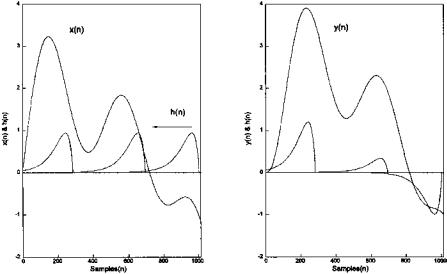
The convolution process is shown schematically in Figure 2.7. The left graph shows the input, x(n) (dashed curve), to a linear system having an impulse response of h(n) (solid line). The right graph of Figure 2.7 shows three partial responses (solid curves) produced by three different infinitely small data segments at N1, N2, and N3. Each partial response is an impulse response scaled by the associated input segment and shifted to the position of that segment. The output of the linear process (right graph, dashed line) is the summation of the individual

FIGURE 2.7 (A) The input, x(n), to a linear system (dashed line) and the impulse response of that system, h(n) (solid line). Three points on the input data sequence are shown: N1, N2, and N3. (B) The partial contributions from the three input data points to the output are impulse responses scaled by the value of the associated input data point (solid line). The overall response of the system, y(n) (dashed line, scaled to fit on the graph), is obtained by summing the contributions from all the input points.

Copyright 2004 by Marcel Dekker, Inc. All Rights Reserved.

impulse responses produced by each of the input data segments. (The output is scaled down to produce a readable plot).

Stated mathematically, the output y(t), to any input, x(t) is given by:

To determine the impulse of each infinitely small data segment, the impulse response is shifted a time τ with respect to the input, then scaled (i.e., multiplied) by the magnitude of the input at that point in time. It does not matter which function, the input or the impulse response, is shifted.* Shifting and multiplication is sometimes referred to as the lag product. For most systems, h(τ) is finite, so the limit of integration is finite. Moreover, a real system can only respond to past inputs, so h(τ) must be 0 for τ < 0 (negative τ implies future times in Eq. (14), although for computer-based operations, where future data may be available in memory, τ can be negative.

For discrete signals, the integration becomes a summation and the convolution equation becomes:

k=1

Again either h(n) or x(n) can be shifted. Also for discrete data, both h(n) and x(n) must be finite (since they are stored in finite memory), so the summation is also finite (where N is the length of the shorter function, usually h(n)).

In signal processing, convolution can be used to implement some of the basic filters described in Chapter 4. Like their analog counterparts, digital filters are just linear processes that modify the input spectra in some desired way (such as reducing noise). As with all linear processes, the filter’s impulse response, h(n), completely describes the filter. The process of sampling used in analog- to-digital conversion can also be viewed in terms of convolution: the sampled output x(n) is just the convolution of the analog signal, x(t), with a very short pulse (i.e., an impulse function) that is periodic with the sampling frequency. Convolution has signal processing implications that extend beyond the determination of input-output relationships. We will show later that convolution in the time domain is equivalent to multiplication in the frequency domain, and vice versa. The former has particular significance to sampling theory as described latter in this chapter.

*Of course, shifting both would be redundant.

Copyright 2004 by Marcel Dekker, Inc. All Rights Reserved.

Covariance and Correlation

The word correlation connotes similarity: how one thing is like another. Mathematically, correlations are obtained by multiplying and normalizing. Both covariance and correlation use multiplication to compare the linear relationship between two variables, but in correlation the coefficients are normalized to fall between zero and one. This makes the correlation coefficients insensitive to variations in the gain of the data acquisition process or the scaling of the variables. However, in many signal processing applications, the variable scales are similar, and covariance is appropriate. The operations of correlation and covariance can be applied to two or more waveforms, to multiple observations of the same source, or to multiple segments of the same waveform. These comparisons between data sequences can also result in a correlation or covariance matrix as described below.

Correlation/covariance operations can not only be used to compare different waveforms at specific points in time, they can also make comparisons over a range of times by shifting one signal with respect the other. The crosscorrelation function is an example of this process. The correlation function is the lagged product of two waveforms, and the defining equation, given here in both continuous and discrete form, is quite similar to the convolution equation above (Eqs. (14) and (15):

k=1

Eqs. (16a) and (16b) show that the only difference in the computation of the crosscorrelation versus convolution is the direction of the shift. In convolution the waveforms are shifted in opposite directions. This produces a causal output: the output function is the creation of past values of the input function (the output is caused by the input). This form of shifting is reflected in the negative sign in Eq. (15). Crosscorrelation shows the similarity between two waveforms at all possible relative positions of one waveform with respect to the other, and it is useful in identifying segments of similarity. The output of Eq. (16) is sometimes termed the raw correlation since there is no normalization involved. Various scalings can be used (such as dividing by N, the number of in the sum), and these are described in the section on MATLAB implementation.

A special case of the correlation function occurs when the comparison is between two waveforms that are one in the same; that is, a function is correlated with different shifts of itself. This is termed the autocorrelation function and it

Copyright 2004 by Marcel Dekker, Inc. All Rights Reserved.

provides a description of how similar a waveform is to itself at various time shifts, or time lags. The autocorrelation function will naturally be maximum for zero lag (n = 0) because at zero lag the comparison is between identical waveforms. Usually the autocorrelation is scaled so that the correlation at zero lag is 1. The function must be symmetric about n = 0, since shifting one version of the same waveform in the negative direction is the same as shifting the other version in the positive direction.

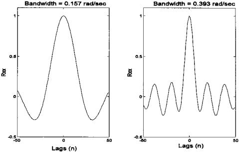
The autocorrelation function is related to the bandwidth of the waveform. The sharper the peak of the autocorrelation function the broader the bandwidth. For example, in white noise, which has infinite bandwidth, adjacent points are uncorrelated, and the autocorrelation function will be nonzero only for zero lag (see Problem 2). Figure 2.8 shows the autocorrelation functions of noise that has been filtered to have two different bandwidths. In statistics, the crosscorrelation and autocorrelation sequences are derived from the expectation operation applied to infinite data. In signal processing, data lengths are finite, so the expec-

FIGURE 2.8 Autocorrelation functions of a random time series with a narrow bandwidth (left) and broader bandwidth (right). Note the inverse relationship between the autocorrelation function and the spectrum: the broader the bandwidth the narrower the first peak. These figures were generated using the code in Example 2.2 below.

Copyright 2004 by Marcel Dekker, Inc. All Rights Reserved.

tation operation becomes summation (with or without normalization), and the crosscorrelation and autocorrelation functions are necessarily estimations.

The crosscovariance function is the same as crosscorrelation function except that the means have been removed from the data before calculation. Accordingly, the equation is a slight modification of Eq. (16b), as shown below:

k=1

The terms correlation and covariance, when used alone (i.e., without the term function), imply operations similar to those described in Eqs. (16) and (17), but without the lag operation. The result will be a single number. For example, the covariance between two functions is given by:

k=1

Of particular interest is the covariance and correlation matrices. These analysis tools can be applied to multivariate data where multiple responses, or observations, are obtained from a single process. A representative example in biosignals is the EEG where the signal consists of a number of related waveforms taken from different positions on the head. The covariance and correlation matrices assume that the multivariate data are arranged in a matrix where the columns are different variables and the rows are different observations of those variables. In signal processing, the rows are the waveform time samples, and the columns are the different signal channels or observations of the signal. The covariance matrix gives the variance of the columns of the data matrix in the diagonals while the covariance between columns is given by the off-diagonals:

An example of the use of the covariance matrix to compare signals is given in the section on MATLAB implementation.

In its usual signal processing definition, the correlation matrix is a normalized version of the covariance matrix. Specifically, the correlation matrix is related to the covariance matrix by the equation:

Copyright 2004 by Marcel Dekker, Inc. All Rights Reserved.

The correlation matrix is a set of correlation coefficients between waveform observations or channels and has a similar positional relationship as in the

Since the diagonals in the correlation matrix give the correlation of a given variable or waveform with itself, they will all equal 1 (rxx(0) = 1), and the off-diagonals will vary between ± 1.

MATLAB Implementation

MATLAB has specific functions for performing convolution, crosscorrelation/ autocorrelation, crossvariance/autocovariance, and construction of the correlation and covariance matrices. To implement convolution in MATLAB, the code is straightforward using the conv function:

y = conv(x,h)

where x and h are vectors containing the waveforms to be convolved and y is the output waveform. The length of the output waveform is equal to the length of x plus the length of h minus 1. This will produce additional data points, and methods for dealing with these extra points are presented at the end of this chapter, along with other problems associated with finite data. Frequently, the additional data points can simply be discarded. An example of the use of this routine is given in Example 2.2. Although the algorithm performs the process defined in equation in Eq. (15), it actually operates in the frequency domain to improve the speed of the operation.

The crosscorrelation and autocorrelation operations are both performed with the same MATLAB routine, with autocorrelation being treated as a special case:

[c,lags] = xcorr(x,y,maxlags,‘options’)

Only the first input argument, x, is required. If no y variable is specified, autocorrelation is performed. The optional argument maxlags specifies the shifting range. The shifted waveform is shifted between ± maxlags, or the default value which is −N + 1 to N − 1 where N is length of the input vector, x. If a y vector is specified then crosscorrelation is performed, and the same shifting range applies. If one of the waveforms the shorter than the other (as is usually

Copyright 2004 by Marcel Dekker, Inc. All Rights Reserved.

the case), it is zero padded (defined and described at the end of this chapter) to be the same length as the longer segment; hence, N would be the length of longer waveform. A number of scaling operations can be specified by the argument options. If options equals biased, the output is divided by 1/N which gives a biased estimate of the crosscorrelation/autocorrelation function. If options equals unbiased, the output is scaled by 1/*N − M* where M is the length of the data output as defined below. Setting options to coeff is used in autocorrelation and scales the autocorrelation function so that the zero lag autocorrelation has a value equal to one. Finally options equals none indicates no scaling, which is the default.

The xcorr function produces an output argument, c, that is a vector of length 2 maxlags + 1 if maxlags is specified or 2N − 1 if the default range is used. The optional output argument, lags, is simply a vector containing the lag values (i.e., a vector of integers ranging between ±maxlags and is useful in plotting.

Autocovariance or crosscovariance is obtained using the xcov function:

[c,lags] = xcov(x,y,maxlags,‘options’)

The arguments are identical to those described above for the xcorr func-

tion.

Correlation or covariance matrices are calculated using the corrcoef or cov functions respectively. Again, the calls are similar for both functions:

Rxx = corrcoef(x)

S = cov(x), or S = cov(x,1);

Without the additional 1 in the calling argument, cov normalizes by N − 1, which provides the best unbiased estimate of the covariance matrix if the observations are from a Gaussian distribution. When the second argument is present, cov normalizes by N which produces the second moment of the observations about their mean.

Example 2.2 shows the use of both the convolution and autocorrelation functions. The program produces autocorrelation functions of noise bandlimited at two different frequencies. To generate the bandlimited (i.e., colored) noise used for the autocorrelation, an impulse response function is generated in the form of sin(x)/x (i.e., the sinc function). We will see in Chapter 4 that this is the impulse response of one type of lowpass filter. Convolution of this impulse response with a white noise sequence is used to generate bandlimited noise. A vector containing Gaussian white noise is produced using the randn routine and the lowpass filter is implemented by convolving the noise with the filter’s im-

Copyright 2004 by Marcel Dekker, Inc. All Rights Reserved.

pulse response. The result is noise bandlimited by the cutoff frequency of the filter. The output of the filter is then processed by the autocorrelation routine to produce the autocorrelation curves shown in Figure 2.8 above. The two figures were obtained for bandlimited noise having bandwidths of π/20 rad/sec and π/8 rad/sec. The variable wc specifies the cutoff frequency of the lowpass filter in the code below. The theory and implementation of a lowpass filter such as used below are presented in Chapter 4.

Example 2.2 Generate bandlimited noise and compute and plot the autocorrelation function for two different bandwidths.

%Example 2.2 and Figure 2.8

%Generate colored noise having two different bandwidths

%and evaluate using autocorrelation.

%

%Compute the impulse response of a lowpass filter

%This type of filter is covered in Chapter 4

Copyright 2004 by Marcel Dekker, Inc. All Rights Reserved.

xlabel(‘Lags(n)’); title([‘Bandwidth =

‘num2str(wc)]);

end

Example 2.3 evaluates the covariance and correlation of sinusoids that are, and are not, orthogonal. Specifically, this example demonstrates the lack of correlation and covariance between sinusoids that are orthogonal such as a sine and cosine at the same frequency and harmonically related sinusoids (i.e., those having multiple frequencies of one another). It also shows correlation and covariance for sinusoids that are not orthogonal such as sines that are not at harmonically related frequencies.

Example 2.3 Generate a data matrix where the columns consist of orthogonal and non-orthogonal sinusoids. Specifically, the data matrix should consist of a 1 Hz sine and a cosine, a 2 Hz sine and cosine, and a 1.5 Hz sine and cosine. The six sinusoids should all be at different amplitudes. The first four sinusoids are orthogonal and should show negligible correlation while the two

1.5Hz sinusoids should show some correlation with the other sinusoids.

%Example 2.3

%Application of the correlation and covariance matrices to

%sinusoids that are orthogonal and non-orthogonal

%

clear all; close all; N = 256;

fs = 256;

n = (1:N)/fs;

%

% Generate the sinusoids as columns of the matrix

The output from this program is a covariance and correlation matrix. The covariance matrix is:

Copyright 2004 by Marcel Dekker, Inc. All Rights Reserved.