Biosignal and Biomedical Image Processing MATLAB based Applications - John L. Semmlow

FIGURE 11.15 Image registration using a transformation developed interactively. The original (reference) image is seen on the left, and the input image in the center. The image after transformation is similar, but not identical to the reference image. The correlation between the two is 0.79. (Original image from the MATLAB Image Processing Toolbox. Copyright 1993–2003, The Math Works, Inc. Reprinted with permission.)

a half-wave sine function of same length. Now take the inverse Fourier transform of this windowed function and plot alongside the original image. Also apply the window in the vertical direction, take the inverse Fourier transform, and plot the resulting image. Do not apply fftshift to the Fourier transform as the inverse Fourier transform routine, ifft2 expects the DC component to be in the upper left corner as fft2 presents it. Also you should take the absolute value at the inverse Fourier transform before display, to eliminate any imaginary components. (The chirp image is square, so you do not have to recompute the half-wave sine function; however, you may want to plot the sine wave to verify that you have a correct half-wave sine function ). You should be able to explain the resulting images. (Hint: Recall the frequency characteristics of the two-point central difference algorithm used for taking the derivative.)

3.Load the blood cell image (blood1.tif). Design and implement your own 3 by 3 filter that enhances vertical edges that go from dark to light. Repeat for a filter that enhances horizontal edges that go from light to dark. Plot the two images along with the original. Convert the first image (vertical edge enhancement) to a binary image and adjust the threshold to emphasize the edges. Plot this image with the others in the same figure. Plot the three-dimensional frequency representations of the two filters together in another figure.

4.Load the chirp image (imchirp.tif) used in Problem 2. Design a onedimensional 64th-order narrowband bandpass filter with cutoff frequencies of 0.1 and 0.125 Hz and apply it the chirp image. Plot the modified image with the original. Repeat for a 128th-order filter and plot the result with the others. (This may take a while to run.) In another figure, plot the three-dimensional frequency representation of a 64th-order filter.

Copyright 2004 by Marcel Dekker, Inc. All Rights Reserved.

5.Produce a movie of the rotating brain. Load frame 16 of the MRI image (mri.tif). Make a multiframe image of the basic image by rotating that image through 360 degrees. Use 36 frames (10 degrees per rotation) to cover the complete 360 degrees. (If your resources permit, you could use 64 frames with 5 degrees per rotation.) Submit a montage plot of those frames that cover the first

90degrees of rotation; i.e., the first eight images (or 16, if you use 64 frames).

6.Back in the 1960’s, people were into “expanding their minds” through meditation, drugs, rock and roll, or other “mind-expanding” experiences. In this problem, you will expand the brain in a movie using an affine transformation. (Note: imresize will not work because it changes the number of pixels in the image and immovie requires that all images have the same dimensions.) Load frame 18 of the MRI image (mri.tif). Make a movie where the brain stretches in and out horizontally from 75% to 150% of normal size. The image will probably exceed the frame size during its larger excursions, but this is acceptable. The image should grow symmetrically about the center (i.e., in both directions.) Use around 24 frames with the latter half of the frames being the reverse of the first as in Example 11.7, so the brain appears to grow then shrink. Submit a montage of the first 12 frames. Note: use some care in getting the range of image sizes to be between 75% and 150%. (Hint: to simplify the computation of the output triangle, it is best to define the input triangle at three of the image corners. Note that all three triangle vertices will have to be modified to stretch the image in both directions, symmetrically about the center.)

7.Produce a spatial transformation movie using a projective transformation. Load a frame of the MRI image (mri.tif, your choice of frame). Use the projective transformation to make a movie of the image as it tilts vertically. Use 24 frames as in Example 11.7: the first 12 will tilt the image back while the rest tilt the image back to its original position. You can use any reasonable transformation that gives a vertical tilt or rotation. Submit a montage of the first 12 images.

8.Load frame 12 of mri.tif and use imrotate to rotate the image by 15 degrees clockwise. Also reduce image contrast of the rotated image by 25%. Use MATLAB’s basic optimization program fminsearch to align the image that has been rotated. (You will need to write a function similar to rescale in Example 11.8 that rotates the image based on the first input parameter, then computes the negative correlation between the rotated image and the original image.)

9.Load a frame of the MRI image (mri.tif) and perform a spatial transformation that first expands the image horizontally by 20% then rotates the image by 20 degrees. Use interactive registration and the MATLAB function cp2tform to transform the image. Use (A) the minimum number of points and (B)

twice the minimum number of points. Compare the correlation between the original and the realigned image using the two different number of reference points.

Copyright 2004 by Marcel Dekker, Inc. All Rights Reserved.

12

Image Segmentation

Image segmentation is the identification and isolation of an image into regions that—one hopes—correspond to structural units. It is an especially important operation in biomedical image processing since it is used to isolate physiological and biological structures of interest. The problems associated with segmentation have been well studied and a large number of approaches have been developed, many specific to a particular image. General approaches to segmentation can be grouped into three classes: pixel-based methods, regional methods, and edgebased methods. Pixel-based methods are the easiest to understand and to implement, but are also the least powerful and, since they operate on one element at time, are particularly susceptible to noise. Continuity-based and edge-based methods approach the segmentation problem from opposing sides: edge-based methods search for differences while continuity-based methods search for similarities.

PIXEL-BASED METHODS

The most straightforward and common of the pixel-based methods is thresholding in which all pixels having intensity values above, or below, some level are classified as part of the segment. Thresholding is an integral part of converting an intensity image to a binary image as described in Chapter 10. Thresholding is usually quite fast and can be done in real time allowing for interactive setting of the threshold. The basic concept of thresholding can be extended to include

Copyright 2004 by Marcel Dekker, Inc. All Rights Reserved.

both upper and lower boundaries, an operation termed slicing since it isolates a specific range of pixels. Slicing can be generalized to include a number of different upper and lower boundaries, each encoded into a different number. An example of multiple slicing was presented in Chapter 10 using the MATLAB gray2slice routine. Finally, when RGB color or pseudocolor images are involved, thresholding can be applied to each color plane separately. The resulting image could be either a thresholded RGB image, or a single image composed of a logical combination (AND or OR) of the three image planes after thresholding. An example of this approach is seen in the problems.

A technique that can aid in all image analysis, but is particularly useful in pixel-based methods, is intensity remapping. In this global procedure, the pixel values are rescaled so as to extend over different maximum and minimum values. Usually the rescaling is linear, so each point is adjusted proportionally with a possible offset. MATLAB supports rescaling with the routine imadjust described below, which also provides a few common nonlinear rescaling options. Of course, any rescaling operation is possible using MATLAB code if the intensity images are of class double, or the image arithmetic routines described in Chapter 10 are used.

Threshold Level Adjustment

A major concern in these pixel-based methods is setting the threshold or slicing level(s) appropriately. Usually these levels are set by the program, although in some situations they can be set interactively by the user.

Finding an appropriate threshold level can be aided by a plot of pixel intensity distribution over the whole image, regardless of whether you adjust the pixel level interactively or automatically. Such a plot is termed the intensity histogram and is supported by the MATLAB routine imhist detailed below. Figure 12.1 shows an x-ray image of the spine image with its associated density histogram. Figure 12.1 also shows the binary image obtained by applying a threshold at a specific point on the histogram. When RGB color images are being analyzed, intensity histograms can be obtained from all three color planes and different thresholds established for each color plane with the aid of the corresponding histogram.

Intensity histograms can be very helpful in selecting threshold levels, not only for the original image, but for images produced by various segmentation algorithms described later. Intensity histograms can also be useful in evaluating the efficacy of different processing schemes: as the separation between structures improves, histogram peaks should become more distinctive. This relationship between separation and histogram shape is demonstrated in Figures 12.2 and, more dramatically, in Figures 12.3 and 12.4.

Copyright 2004 by Marcel Dekker, Inc. All Rights Reserved.

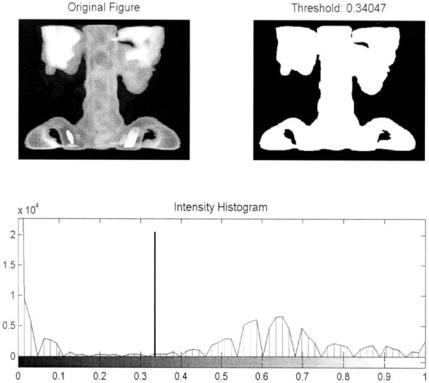
FIGURE 12.1 An image of bone marrow, upper left, and its associated intensity histogram, lower plot. The upper right image is obtained by thresholding the original image at a value corresponding to the vertical line on the histogram plot. (Original image from the MATLAB Image Processing Toolbox. Copyright 1993– 2003, The Math Works, Inc. Reprinted with permission.)

Intensity histograms contain no information on position, yet it is spatial information that is of prime importance in problems of segmentation, so some strategies have been developed for determining threshold(s) from the histogram (Sonka et al. 1993). If the intensity histogram is, or can be assumed as, bimodal (or multi-modal), a common strategy is to search for low points, or minima, in the histogram. This is the strategy used in Figure 12.1, where the threshold was set at 0.34, the intensity value at which the histogram shows an approximate minimum. Such points represent the fewest number of pixels and should produce minimal classification errors; however, the histogram minima are often difficult to determine due to variability.

Copyright 2004 by Marcel Dekker, Inc. All Rights Reserved.

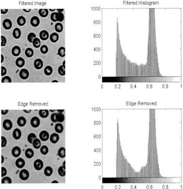
FIGURE 12.2 Image of bloods cells with (upper) and without (lower) intermediate boundaries removed. The associated histograms (right side) show improved separability when the boundaries are eliminated. The code that generated these images is given in Example 12.1. (Original image reprinted with permission from the Image Processing Handbook 2nd edition. Copyright CRC Press, Boca Raton, Florida.)

An approach to improve the determination of histogram minima is based on the observation that many boundary points carry values intermediate to the values on either side of the boundary. These intermediate values will be associated with the region between the actual boundary values and may mask the optimal threshold value. However, these intermediate points also have the highest gradient, and it should be possible to identify them using a gradient-sensitive filter, such as the Sobel or Canny filter. After these boundary points are identified, they can be eliminated from the image, and a new histogram is computed with a distribution that is possibly more definitive. This strategy is used in

Copyright 2004 by Marcel Dekker, Inc. All Rights Reserved.

FIGURE 12.3 Thresholded blood cell images. Optimal thresholds were applied to the blood cell images in Figure 12.2 with (left) and without (right) boundaries pixel masked. Fewer inappropriate pixels are seen in the right image.

Example 12.1, and Figure 12.2 shows images and associated histograms before and after removal of boundary points as identified using Canny filtering. The reduction in the number of intermediate points can be seen in the middle of the histogram (around 0.45). As shown in Figure 12.3, this leads to slightly better segmentation of the blood cells.

Another histogram-based strategy that can be used if the distribution is bimodal is to assume that each mode is the result of a unimodal, Gaussian distribution. An estimate is then made of the underlying distributions, and the point at which the two estimated distributions intersect should provide the optimal threshold. The principal problem with this approach is that the distributions are unlikely to be truly Gaussian.

A threshold strategy that does not use the histogram is based on the concept of minimizing the variance between presumed foreground and background elements. Although the method assumes two different gray levels, it works well even when the distribution is not bimodal (Sonka et al., 1993). The approach uses an iterative process to find a threshold that minimizes the variance between the intensity values on either side of the threshold level (Outso’s method). This approach is implemented using the MATLAB routine grayslice (see Example 12.1).

A pixel-based technique that provides a segment boundary directly is contour mapping. Contours are lines of equal intensity, and in a continuous image they are necessarily continuous: they cannot end within the image, although

Copyright 2004 by Marcel Dekker, Inc. All Rights Reserved.

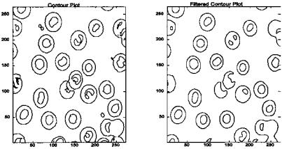
FIGURE 12.4 Contour maps drawn from the blood cell image of Figures 12.2 and 12.3. The right image was pre-filtered with a Gaussian lowpass filter (alpha = 3) before the contour lines were drawn. The contour values were set manually to provide good images.

they can branch or loop back on themselves. In digital images, these same properties exist but the value of any given contour line will not generally equal the values of the pixels it traverses. Rather, it usually reflects values intermediate between adjacent pixels. To use contour mapping to identify image structures requires accurate setting of the contour levels, and this carries the same burdens as thresholding. Nonetheless, contour maps do provide boundaries directly, and, if subpixel interpolation is used in establishing the contour position, they may be spatially more accurate. Contour maps are easy to implement in MATLAB, as shown in the next section on MATLAB Implementation. Figure 12.4 shows contours maps for the blood cell images shown in Figure 12.2. The right image was pre-filtered with a Gaussian lowpass filter which reduces noise slightly and improves the resultant contour image.

Pixel-based approaches can lead to serious errors, even when the average intensities of the various segments are clearly different, due to noise-induced intensity variation within the structure. Such variation could be acquired during image acquisition, but could also be inherent in the structure itself. Figure 12.5 shows two regions with quite different average intensities. Even with optimal threshold selection, many inappropriate pixels are found in both segments due to intensity variations within the segments Fig 12.3 (right). Techniques for improving separation in such images are explored in the sections on continuitybased approaches.

Copyright 2004 by Marcel Dekker, Inc. All Rights Reserved.

FIGURE 12.5 An image with two regions having different average gray levels. The two regions are clearly distinguishable; however, using thresholding alone, it is not possible to completely separate the two regions because of noise.

MATLAB Implementation

Some of the routines for implementing pixel-based operations such as im2bw and grayslice have been described in preceding chapters. The image intensity histogram routine is produced by imhist without the output arguments:

[counts, x] = imhist(I, N);

where counts is the histogram value at a given x, I is the image, and N is an optional argument specifying the number of histogram bins (the default is 255). As mentioned above, imhist is usually invoked without the output arguments, count and x, to produce a plot directly.

The rescale routine is:

I_rescale = imscale(I, [low high], [bottom top], gamma);

where I_rescale is the rescaled output image, I is the input image. The range between low and high in the input image is rescaled to be between bottom and top in the output image.

Several pixel-based techniques are presented in Example 12.1.

Example 12.1 An example of segmentation using pixel-based methods. Load the image of blood cells, and display along with the intensity histogram. Remove the edge pixels from the image and display the histogram of this modi-

Copyright 2004 by Marcel Dekker, Inc. All Rights Reserved.

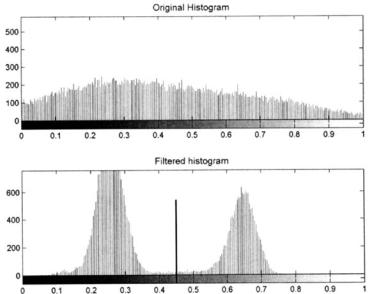
FIGURE 12.6A Histogram of the image shown in Figure 12.3 before (upper) and after (lower) lowpass filtering. Before filtering the two regions overlap to such an extend that they cannot be identified. After lowpass filtering, the two regions are evident, and the boundary found by minimum variance is shown. The application of this boundary to the filtered image results in perfect separation as shown in Figure 12.4B.

fied image. Determine thresholds using the minimal variance iterative technique described above, and apply this approach to threshold both images. Display the resultant thresholded images.

Solution To remove the edge boundaries, first identify these boundaries using an edge detection scheme. While any of the edge detection filters described previously can be used, this application will use the Canny filter as it is most robust to noise. This filter is implemented as an option of MATLAB’s edge routine, which produces a binary image of the boundaries. This binary image will be converted to a boundary mask by inverting the image using imcomplement. After inversion, the edge pixels will be zero while all other pixels will be one. Multiplying the original image by the boundary mask will produce an image in which the boundary points are removed (i.e., set to zero, or black). All the images involved in this process, including the original image, will then be plotted.

Copyright 2004 by Marcel Dekker, Inc. All Rights Reserved.