Biosignal and Biomedical Image Processing MATLAB based Applications - John L. Semmlow

the map variables. (This problem actually occurred in this example when the sliced array was displayed as an Indexed variable.) The easiest solution to this potential problem is to convert the image to RGB before calling imshow as was done in this example.

Many images that are grayscale can benefit from some form of color coding. With the RGB format, it is easy to highlight specific features of a grayscale image by placing them in a specific color plane. The next example illustrates the use of color planes to enhance features of a grayscale image.

Example 10.5 In this example, brightness levels of a grayscale image that are 50% or less are coded into shades of blue, and those above are coded into shades of red. The grayscale image is first put in double format so that the maximum range is 0 to 1. Then each pixel is tested to be greater than 0.5. Pixel values less that 0.5 are placed into the blue image plane of an RGB image (i.e., the third plane). These pixel values are multiplied by two so they take up the full range of the blue plane. Pixel values above 0.5 are placed in the red plane (plane 1) after scaling to take up the full range of the red plane. This image is displayed in the usual way. While it is not reproduced in color here, a homework problem based on these same concepts will demonstrate pseudocolor.

%Example 10.5 and Figure 10.7 Example of the use of pseudocolor

%Load frame 17 of the MRI image (mri.tif)

%from the Image Processing Toolbox in subdirectory ‘imdemos’.

FIGURE 10.7 Frame 17 of the MRI image given in Figure 10.5 plotted directly and in pseudocolor using the code in Example 10.5. (Original image from MATLAB). Copyright 1993–2003, The Math Works, Inc. Reprinted with permission.

Copyright 2004 by Marcel Dekker, Inc. All Rights Reserved.

%Display a pseudocolor image in which all values less that 50%

%maximum are in shades of blue and values above are in shades

%of red.

%

clear all; close all; frame = 17;

[I(:,:,1,1), map ] = imread(’mri.tif’, frame);

% Now check to see if image is Indexed (in fact ’whos’ shows it is).

imshow(I); title(’Original’); subplot(1,2,2);

imshow(RGB) title(’Pseudocolor’);

The pseudocolor image produced by this code is shown in Figure 10.7. Again, it will be necessary to run the example to obtain the actual color image.

ADVANCED PROTOCOLS: BLOCK PROCESSING

Many of the signal processing techniques presented in previous chapters operated on small, localized groups of data. For example, both FIR and adaptive filters used data samples within the same general neighborhood. Many image processing techniques also operate on neighboring data elements, except the neighborhood now extends in two dimensions, both horizontally and vertically. Given this extension into two dimensions, many operations in image processing are quite similar to those in signal processing. In the next chapter, we examine both two-dimensional filtering using two-dimensional convolution and the twodimensional Fourier transform. While many image processing operations are conceptually the same as those used on signal processing, the implementation

Copyright 2004 by Marcel Dekker, Inc. All Rights Reserved.

is somewhat more involved due to the additional bookkeeping required to operate on data in two dimensions. The MATLAB Image Processing Toolbox simplifies much of the tedium of working in two dimensions by introducing functions that facilitate two-dimensional block, or neighborhood operations. These block processing operations fall into two categories: sliding neighborhood operations and distinct block operation. In sliding neighborhood operations, the block slides across the image as in convolution; however, the block must slide in both horizontal and vertical directions. Indeed, two-dimensional convolution described in the next chapter is an example of one very useful sliding neighborhood operation. In distinct block operations, the image area is divided into a number of fixed groups of pixels, although these groups may overlap. This is analogous to the overlapping segments used in the Welch approach to the Fourier transform described in Chapter 3. Both of these approaches to dealing with blocks of localized data in two dimensions are supported by MATLAB routines.

Sliding Neighborhood Operations

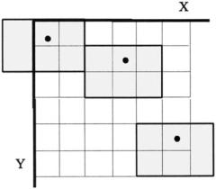
The sliding neighborhood operation alters one pixel at a time based on some operation performed on the surrounding pixels; specifically those pixels that lie within the neighborhood defined by the block. The block is placed as symmetrically as possible around the pixel being altered, termed the center pixel (Figure 10.8). The center pixel will only be in the center if the block is odd in both

FIGURE 10.8 A 3-by-2 pixel sliding neighborhood block. The block (gray area), is shown in three different positions. Note that the block sometimes falls off the picture and padding (usually zero padding) is required. In actual use, the block slides, one element at a time, over the entire image. The dot indicates the center pixel.

Copyright 2004 by Marcel Dekker, Inc. All Rights Reserved.

dimensions, otherwise the center pixel position favors the left and upper sides of the block (Figure 10.8).* Just as in signal processing, there is a problem that occurs at the edge of the image when a portion of the block will extend beyond the image (Figure 10.8, upper left block). In this case, most MATLAB sliding block functions automatically perform zero padding for these pixels. (An exception, is the imfilter routine described in the next capter.)

The MATLAB routines conv2 and filter2 are both siding neighborhood operators that are directly analogous to the one dimensional convolution routine, conv, and filter routine, filter. These functions will be discussed in the next chapter on image filtering. Other two-dimensional functions that are directly analogous to their one-dimensional counterparts include: mean2, std2, corr2, and fft2. Here we describe a general sliding neighborhood routine that can be used to implement a wide variety of image processing operations. Since these operations can be—but are not necessarily—nonlinear, the function has the name nlfilter, presumably standing for nonlinear filter. The calling structure is:

I1 = nlfilter(I, [M N], func, P1, P2, ...);

where I is the input image array, M and N are the dimensions of the neighborhood block (horizontal and vertical), and func specifies the function that will operate over the block. The optional parameters P1, P2, . . . , will be passed to the function if it requires input parameters. The function should take an M by N input and must produce a single, scalar output that will be used for the value of the center pixel. The input can be of any class or data format supported by the function, and the output image array, I1, will depend on the format provided by the routine’s output.

The function may be specified in one of three ways: as a string containing the desired operation, as a function handle to an M-file, or as a function established by the routine inline. The first approach is straightforward: simply embed the function operation, which could be any appropriate MATLAB statment(s), within single quotes. For example:

I1 = nlfilter(I, [3 3], ‘mean2’);

This command will slide a 3 by 3 moving average across the image producing a lowpass filtered version of the original image (analogous to an FIR filter of [1/3 1/3 1/3] ). Note that this could be more effectively implemented using the filter routines described in the next chapter, but more complicated, perhaps nonlinear, operations could be included within the quotes.

*In MATLAB notation, the center pixel of an M by N block is located at: floor(([M N] 1)/2).

Copyright 2004 by Marcel Dekker, Inc. All Rights Reserved.

The use of a function handle is shown in the code:

I1 = nlfilter(I, [3 3], @my_function);

where my_function is the name of an M-file function. The function handle @my_function contains all the information required by MATLAB to execute the function. Again, this file should produce a single, scalar output from an M by N input, and it has the possibility of containing input arguments in addition to the block matrix.

The inline routine has the ability to take string text and convert it into a function for use in nlfilter as in this example string:

F= inline(‘2*x(2,2) -sum( x(1:3,1))/3- sum(x(1:3,3))/3

-x(1,2)—x(3,2)’);

I1 = nlfilter(I, [3 3], F);

Function inline assumes that the input variable is x, but it also can find other variables based on the context and it allows for additional arguments, P1, P2, . . . (see associated help file). The particular function shown above would take the difference between the center point and its 8 surrounding neighbors, performing a differentiator-like operation. There are better ways to perform spatial differentiation described in the next chapter, but this form will be demonstrated as one of the operations in Example 10.6 below.

Example 10.6 Load the image of blood cells in blood.tiff in MATLAB’s image files. Convert the image to class intensity and double format. Perform the following sliding neighborhood operations: averaging over a 5 by 5 sliding block, differencing (spatial differentiation) using the function, F, above; and vertical boundary detection using a 2 by 3 vertical differencer. This differencer operator subtracts a vertical set of three left hand pixels from the three adjacent right hand pixels. The result will be a brightening of vertical boundaries that go from dark to light and a darkening of vertical boundaries that go from light to dark. Display all the images in the same figure including the original. Also include binary images of the vertical boundary image thresholded at two different levels to emphasize the left and right boundaries.

%Example 10.6 and Figure 10.9

%Demonstration of sliding neighborhood operations

%Load image of blood cells, blood.tiff from the Image Processing

%Toolbox in subdirectory imdemos.

%Use a sliding 3 by 3 element block to perform several sliding

%neighborhood operations including taking the average over the

%block, implementing the function ’F’ in the example

Copyright 2004 by Marcel Dekker, Inc. All Rights Reserved.

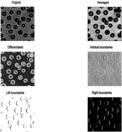
FIGURE 10.9 A variety of sliding neighborhood operations carried out on an image of blood cells. (Original reprinted with permission from The Image Processing Handbook, 2nd ed. Copyright CRC Press, Boca Raton, Florida.)

%above, and implementing a function that enhances vertical

%boundaries.

%Display the original and all modification on the same plot

clear all; close all;

[I map] = imread(’blood1.tif’);% Input image

%Since image is stored in tif format, it could be in either uint8

%or uint16 format (although the ’whos’ command shows it is in

%uint8).

Copyright 2004 by Marcel Dekker, Inc. All Rights Reserved.

%The specific data format will not matter since the format will

%be converted to double either by ’ind2gray,’ if it is an In-

%dexed image or by ‘im2gray’ if it is not.

%

if isempty(map) == 0

I = ind2gray(I,map);

end

I = im2double(I);

%

%Perform the various sliding neighborhood operations.

%Averaging

I_avg = nlfilter(I,[5 5], ’mean2’);

%

% Differencing

F = inline(’x(2,2)—sum(x(1:3,1))/3- sum(x(1:3,3))/3 - ...

x(1,2)—x(3,2)’);

I_diff = nlfilter(I, [3 3], F);

%

% Vertical boundary detection

F1 = inline (’sum(x(1:3,2))—sum(x(1:3,1))’); I_vertical = nlfilter(I,[3 2], F1);

%

% Rescale all arrays I_avg = mat2gray(I_avg);

I_diff = mat2gray(I_diff); I_vertical = mat2gray(I_vertical);

%

subplot(3,2,1); % Display all images in a single % plot

imshow(I);

title(’Original’);

subplot(3,2,2); imshow(I_avg); title(’Averaged’);

subplot(3,2,3); imshow(I_diff); title(’Differentiated’);

subplot(3,2,4); imshow(I_vertical); title(’Vertical boundaries’);

subplot(3,2,5);

bw = im2bw(I_vertical,.6); % Threshold data, low threshold imshow(bw);

Copyright 2004 by Marcel Dekker, Inc. All Rights Reserved.

title(’Left boundaries’);

subplot(3,2,6);

bw1 = im2bw(I_vertical,.8); % Threshold data, high

% threshold

imshow(bw1);

title(’Right boundaries’);

The code in Example 10.6 produces the images in Figure 10.9. These operations are quite time consuming: Example 10.6 took about 4 minutes to run on a 500 MHz PC. Techniques for increasing the speed of Sliding Operations can be found in the help file for colfilt. The vertical boundaries produced by the 3 by 2 sliding block are not very apparent in the intensity image, but become quite evident in the thresholded binary images. The averaging has improved contrast, but the resolution is reduced so that edges are no longer distinct.

Distinct Block Operations

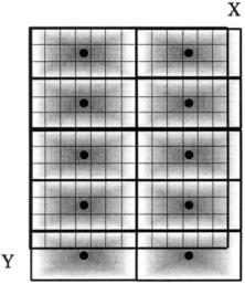
All of the sliding neighborhood options can also be implemented using configurations of fixed blocks (Figure 10.10). Since these blocks do not slide, but are

FIGURE 10.10 A 7-by-3 pixel distinct block. As with the sliding neighborhood block, these fixed blocks can fall off the picture and require padding (usually zero padding). The dot indicates the center pixel although this point usually has little significance in this approach.

Copyright 2004 by Marcel Dekker, Inc. All Rights Reserved.

fixed with respect to the image (although they may overlap), they will produce very different results. The MATLAB function for implementing distinct block operations is similar in format to the sliding neighborhood function:

I1 = blkproc(I, [M N], [Vo Ho], func);

where M and N specify the vertical and horizontal size of the block, Vo and Ho are optional arguments that specify the vertical and horizontal overlap of the block, func is the function that operates on the block, I is the input array, and I1 is the output array. As with nlfilter the data format of the output will depend on the output of the function. The function is specified in the same manner as described for nlfilter; however the function output will be different.

Function outputs for sliding neighborhood operations had to be single scalars that then became the value of the center pixel. In distinct block operations, the block does not move, so the function output will normally produce values for every pixel in the block. If the block produces a single output, then only the center pixel of each block will contain a meaningful value. If the function is an operation that normally produces a single value, the output of this routine can be expanded by multiplying it by an array of ones that is the same size as the block This will place that single output in every pixel in the block:

I1 = blkproc(I [4 5], ‘std2 * ones(4,5)’);

In this example the output of the MATLAB function std2 is placed into a 4 by 5 array and this becomes the output of the function, an array the same size as the block. It is also possible to use the inline function to describe the function:

F = inline(‘std2(x) * ones(size(x))’);

I1 = blkproc(I, [4 5], F);

Of course, it is possible that certain operations could produce a different output for each pixel in the block. An example of block processing is given in Example 10.7.

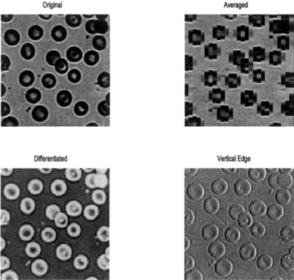
Example 10.7 Load the blood cell image used in Example 10.6 and perform the following distinct block processing operations: 1) Display the average for a block size of 8 by 8; 2) For a 3 by 3 block, perform the differentiator operation used in Example 10.6; and 3) Apply the vertical boundary detector form Example 10.6 to a 3 by 3 block. Display all the images including the original in a single figure.

Copyright 2004 by Marcel Dekker, Inc. All Rights Reserved.

%Example 10.7 and Figure 10.11

%Demonstration of distinct block operations

%Load image of blood cells used in Example 10.6

%Use a 8 by 8 distinct block to get averages for the entire block

%Apply the 3 by 3 differentiator from Example 10.6 as a distinct

%block operation.

%Apply a 3 by 3 vertical edge detector as a block operation

%Display the original and all modification on the same plot

%

..... Image load, same as in Example 10.6.......

%

FIGURE 10.11 The blood cell image of Example 10.6 processed using three Distinct block operations: block averaging, block differentiation, and block vertical edge detection. (Original image reprinted from The Image Processing Handbook, 2nd edition. Copyright CRC Press, Boca Raton, Florida.)

Copyright 2004 by Marcel Dekker, Inc. All Rights Reserved.