Biosignal and Biomedical Image Processing MATLAB based Applications - John L. Semmlow

dimension of the output is the sum of the two matrix lengths along that dimension minus one. Hence, if the two matrices have sizes I1(M1, N1) and h(M2, N2), the output size is: I2(M1 M2 − 1, N2 N2 − 1). If shape is ‘valid’, then any pixel evaluation that requires image padding is ignored and the size of the output image is: Ic(M1M2 1, N1N2 1). Finally, if shape is ‘same’ the size of the output matrix is the same size as I1; that is: I2(M1, N1). These options allow a great deal in flexibility and can simplify the use of two-dimen- sional convolution; for example, the ‘same’ option can eliminate the need for dealing with the additional points generated by convolution.

Two-dimensional correlation is implemented with the routine ‘imfilter’ that provides even greater flexibility and convenience in dealing with size and boundary effects. The calling structure of this routine is given in the next page.

I2 = imfilter(I1, h, options);

where again I1 and h are the input matrices and options can include up to three separate control options. One option controls the size of the output array using the same terms as in ‘conv2’ above: ‘same’ and ‘full’ (‘valid’ is not valid in this routine!). With ‘imfilter’ the default output size is ‘same’ (not ‘full’), since this is the more likely option in image analysis. The second possible option controls how the edges are treated. If a constant is given, then the edges are padded with the value of that constant. The default is to use a constant of zero (i.e., standard zero padding). The boundary option ‘symmetric’ uses a mirror reflection of the end points as shown in Figure 2.10. Similarly the option ‘circular’ uses periodic extension also shown in Figure 2.10. The last boundary control option is ‘replicate’, which pads using the nearest edge pixel. When the image is large, the influence of the various border control options is subtle, as shown in Example 11.4. A final option specifies the use of convolution instead of correlation. If this option is activated by including the argument conv, imfilter is redundant with ‘conv2’ except for the options and defaults. The imfilter routine will accept all of the data format and types defined in the previous chapter and produces an output in the same format; however, filtering is not usually appropriate for indexed images. In the case of RGB images, imfilter operates on all three image planes.

Filter Design

The MATLAB Image Processing Toolbox provides considerable support for generating the filter coefficients.* A number of filters can be generated using MATLAB’s fspecial routine:

*Since MATLAB’s preferred implementation of image filters is through correlation, not convolution, MATLAB’s filter design routines generate correlation kernels. We use the term “filter coefficient” for either kernel format.

Copyright 2004 by Marcel Dekker, Inc. All Rights Reserved.

h = fspecial(type, parameters);

where type specifies a specific filter and the optional parameters are related to the filter selected. Filter type options include: ‘gaussian’, ‘disk’, ‘sobel’,

‘prewitt’, ‘laplacian’, ‘log’, ‘average’, and ‘unsharp’. The ‘gaussian’ option produces a Gaussian lowpass filter. The equation for a Gaussian filter is similar to the equation for the gaussian distribution:

This filter has particularly desirable properties when applied to an image: it provides an optimal compromise between smoothness and filter sharpness. The MATLAB routine for this filter accepts two parameters: the first specifies the filter size (the default is 3) and the second the value of sigma. The value of sigma will influence the cutoff frequency while the size of the filter determines the number of pixels over which the filter operates. In general, the size should be 3–5 times the value of sigma.

Both the ‘sobel’ and ‘prewitt’ options produce a 3 by 3 filter that enhances horizontal edges (or vertical if transposed). The ‘unsharp’ filter produces a contrast enhancement filter. This filter is also termed unsharp masking because it actually suppresses low spatial frequencies where the low frequencies are presumed to be the unsharp frequencies. In fact, it is a special highpass filter. This filter has a parameter that specifies the shape of the highpass characteristic. The ‘average’ filter simply produces a constant set of weights each of which equals 1/N, where N = the number of elements in the filter (the default size of this filter is 3 by 3, in which case the weights are all 1/9 = 0.1111). The filter coefficients for a 3 by 3 Gaussian lowpass filter (sigma = 0.5) and the unsharpe filter (alpha = 0.2) are shown below:

The Laplacian filter is used to take the second derivative of an image: ∂2 /∂x. The log filter is actually the log of Gaussian filter and is used to take the first derivative, ∂ /∂x, of an image.

MATLAB also provides a routine to transform one-dimensional FIR filters, such as those described in Chapter 4, into two-dimensional filters. This approach is termed the frequency transform method and preserves most of the characteristics of the one-dimensional filter including the transition bandwidth and ripple features. The frequency transformation method is implemented using:

h = ftrans2(b);

Copyright 2004 by Marcel Dekker, Inc. All Rights Reserved.

where h are the output filter coefficients (given in correlation kernel format), and b are the filter coefficients of a one-dimensional filter. The latter could be produced by any of the FIR routines described in Chapter 4 (i.e., fir1, fir2, or remez). The function ftrans2 can take an optional second argument that specifies the transformation matrix, the matrix that converts the one-dimensional coefficients to two dimensions. The default transformation is the McClellan transformation that produces a nearly circular pattern of filter coefficients. This approach brings a great deal of power and flexibility to image filter design since it couples all of the FIR filter design approaches described in Chapter 4 to image filtering.

The two-dimensional Fourier transform described above can be used to evaluate the frequency characteristics of a given filter. In addition, MATLAB supplies a two-dimensional version of freqz, termed freqz2, that is slightly more convenient to use since it also handles the plotting. The basic call is:

[H fx fy] = freqz2(h, Ny, Nx);.

where h contains the two-dimensional filter coefficients and Nx and Ny specify the size of the desired frequency plot. The output argument, H, contains the twodimensional frequency spectra and fx and fy are plotting vectors; however, if freqz2 is called with no output arguments then it generates the frequency plot directly. The examples presented below do not take advantage of this function, but simply use the two-dimensional Fourier transform for filter evaluation.

Example 11.2 This is an example of linear filtering using two of the filters in fspecial. Load one frame of the MRI image set (mri.tif) and apply the sharpening filter, hunsharp, described above. Apply a horizontal Sobel filter, hSobel, (also shown above), to detect horizontal edges. Then apply the Sobel filter to detect the vertical edges and combine the two edge detectors. Plot both the horizontal and combined edge detectors.

Solution To generate the vertical Sobel edge detector, simply transpose the horizontal Sobel filter. While the two Sobel images could be added together using imadd, the program below first converts both images to binary then combines them using a logical or. This produces a more dramatic black and white image of the boundaries.

%Example 11.2 and Figure 11.4A and B

%Example of linear filtering using selected filters from the

%MATLAB ’fspecial’ function.

%Load one frame of the MRI image and apply the 3 by 3 “unshape”

%contrast enhancement filter shown in the text. Also apply two

Copyright 2004 by Marcel Dekker, Inc. All Rights Reserved.

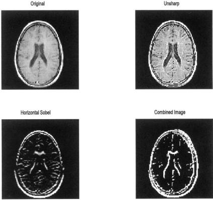
FIGURE 11.4A MRI image of the brain before and after application of two filters from MATLAB’s fspecial routine. Upper right: Image sharpening using the filter unsharp. Lower images: Edge detection using the sobel filter for horizontal edges (left) and for both horizontal and vertical edges (right). (Original image from MATLAB. Image Processing Toolbox. Copyright 1993–2003, The Math Works, Inc. Reprinted with permission.)

%3 by 3 Sobel edge detector filters to enhance horizontal and

%vertical edges.

%Combine the two edge detected images

%

clear all; close all;

%

frame = 17; % Load MRI frame 17 [I(:,:,:,1), map ] = imread(’mri.tif’, frame);

Copyright 2004 by Marcel Dekker, Inc. All Rights Reserved.

FIGURE 11.4B Frequency characteristics of the unsharp and Sobel filters used in Example 11.2.

%

% Combine by converting to binary and or-ing together

I_sobel_combined = im2bw(I_sobel_horin) * ...

im2bw(I_sobel_vertical);

%

subplot(2,2,1); imshow(I); % Plot the images title(’Original’);

subplot(2,2,2); imshow(I_unsharp); title(’Unsharp’);

subplot(2,2,3); imshow(I_sobel_horin);

Copyright 2004 by Marcel Dekker, Inc. All Rights Reserved.

title(’Horizontal Sobel’); subplot(2,2,4); imshow(I_sobel_combined);

title(’Combined Image’); figure;

%

%Now plot the unsharp and Sobel filter frequency

%characteristics

F= fftshift(abs(fft2(h_unsharp,32,32))); subplot(1,2,1); mesh(1:32,1:32,F);

title(’Unsharp Filter’); view([-37,15]);

%

F = fftshift(abs(fft2(h_s,32,32))); subplot(1,2,2); mesh(1:32,1:32,F);

title(’Sobel Filter’); view([-37,15]);

The images produced by this example program are shown below along with the frequency characteristics associated with the ‘unsharp’ and ‘sobel’ filter. Note that the ‘unsharp’ filter has the general frequency characteristics of a highpass filter, that is, a positive slope with increasing spatial frequencies (Figure 11.4B). The double peaks of the Sobel filter that produce edge enhancement are evident in Figure 11.4B. Since this is a magnitude plot, both peaks appear as positive.

In Example 11.3, routine ftrans2 is used to construct two-dimensional filters from one-dimensional FIR filters. Lowpass and highpass filters are constructed using the filter design routine fir1 from Chapter 4. This routine generates filter coefficients based on the ideal rectangular window approach described in that chapter. Example 11.3 also illustrates the use of an alternate padding technique to reduce the edge effects caused by zero padding. Specifically, the ‘replicate’ option of imfilter is used to pad by repetition of the last (i.e., image boundary) pixel value. This eliminates the dark border produced by zero padding, but the effect is subtle.

Example 11.3 Example of the application of standard one-dimensional FIR filters extended to two dimensions. The blood cell images (blood1.tif) are loaded and filtered using a 32 by 32 lowpass and highpass filter. The onedimensional filter is based on the rectangular window filter (Eq. (10), Chapter 4), and is generated by fir. It is then extended to two dimensions using ftrans2.

%Example 11.3 and Figure 11.5A and B

%Linear filtering. Load the blood cell image

%Apply a 32nd order lowpass filter having a bandwidth of .125

%fs/2, and a highpass filter having the same order and band-

%width. Implement the lowpass filter using ‘imfilter’ with the

Copyright 2004 by Marcel Dekker, Inc. All Rights Reserved.

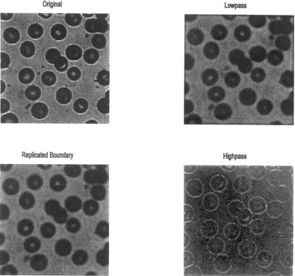
FIGURE 11.5A Image of blood cells before and after lowpass and highpass filtering. The upper lowpass image (upper right) was filtered using zero padding, which produces a slight black border around the image. Padding by extending the edge pixel eliminates this problem (lower left). (Original Image reprinted with permission from The Image Processing Handbook, 2nd edition. Copyright CRC Press, Boca Raton, Florida.)

%zero padding (the default) and with replicated padding

%(extending the final pixels).

%Plot the filter characteristics of the high and low pass filters

%Load the image and transform if necessary

Copyright 2004 by Marcel Dekker, Inc. All Rights Reserved.

FIGURE 11.5B Frequency characteristics of the lowpass (left) and highpass (right) filters used in Figure 11.5A.

I_highpass = imfilter(I, h_hp);

I_highpass = mat2gray(I_highpass);

%

........plot the images and filter characteristics as in

Example 11.2.......

The figures produced by this program are shown below (Figure 11.5A and B). Note that there is little difference between the image filtered using zero padding and the one that uses extended (‘replicate’) padding. The highpass filtered image shows a slight derivative-like characteristic that enhances edges. In the plots of frequency characteristics, Figure 11.5B, the lowpass and highpass filters appear to be circular, symmetrical, and near opposites.

The problem of aliasing due to downsampling was discussed above and

Copyright 2004 by Marcel Dekker, Inc. All Rights Reserved.

demonstrated in Figure 11.1. Such problems could occur whenever an image is displayed in a smaller size that will require fewer pixels, for example when the size of an image is reduced during reshaping of a computer window. Lowpass filtering can be, and is, used to prevent aliasing when an image is downsized. In fact, MATLAB automatically performs lowpass filtering when downsizing an image. Example 11.4 demonstrates the ability of lowpass filtering to reduce aliasing when downsampling is performed.

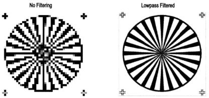
Example 11.4 Use lowpass filtering to reduce aliasing due to downsampling. Load the radial pattern (‘testpat1.png’) and downsample by a factor of six as was done in Figure 11.1. In addition, downsample that image by the same amount, but after it has been lowpass filtered. Plot the two downsampled images side-by-side. Use a 32 by 32 FIR rectangular window lowpass filter. Set the cutoff frequency to be as high as possible and still eliminate most of the aliasing.

%Example 11.4 and Figure 11.6

%Example of the ability of lowpass filtering to reduce aliasing.

%Downsample the radial pattern with and without prior lowpass

%filtering.

%Use a cutoff frequency sufficient to reduce aliasing.

FIGURE 11.6 Two images of the radial pattern shown in Figure 11.1 after downsampling by a factor of 6. The right-hand image was filtered by a lowpass filter before downsampling.

Copyright 2004 by Marcel Dekker, Inc. All Rights Reserved.

%

[Imap] = imread(’testpat1.png’); % Load image

title(’No Filtering’);

% Downsample filtered image and display I_lowass = I_lowpass(1:dwn: M,1:dwn:N); subplot(1,2,2); imshow(I_lowpass);

title (’Lowpass Filtered’);

The lowpass cutoff frequency used in Example 11.5 was determined empirically. Although the cutoff frequency was fairly high ( fS/4), this filter still produced substantial reduction in aliasing in the downsampled image.

SPATIAL TRANSFORMATIONS

Several useful transformations take place entirely in the spatial domain. Such transformations include image resizing, rotation, cropping, stretching, shearing, and image projections. Spatial transformations perform a remapping of pixels and often require some form of interpolation in addition to possible anti-aliasing. The primary approach to anti-aliasing is lowpass filtering, as demonstrated above. For interpolation, there are three methods popularly used in image processing, and MATLAB supports all three. All three interpolation strategies use the same basic approach: the interpolated pixel in the output image is the weighted sum of pixels in the vicinity of the original pixel after transformation. The methods differ primarily in how many neighbors are considered.

As mentioned above, spatial transforms involve a remapping of one set of pixels (i.e., image) to another. In this regard, the original image can be considered as the input to the remapping process and the transformed image is the output of this process. If images were continuous, then remapping would not require interpolation, but the discrete nature of pixels usually necessitates remapping.* The simplest interpolation method is the nearest neighbor method in which the output pixel is assigned the value of the closest pixel in the transformed image, Figure 11.7. If the transformed image is larger than the original and involves more pixels, then a remapped input pixel may fall into two or

*A few transformations may not require interpolation such as rotation by 90 or 180 degrees.

Copyright 2004 by Marcel Dekker, Inc. All Rights Reserved.