Biosignal and Biomedical Image Processing MATLAB based Applications - John L. Semmlow

%Perform the various distinct block operations.

%Average of the image

I_avg = blkproc(I,[10 10], ’mean2 * ones(10,10)’);

%

% Deferentiator—place result in all blocks

F= inline(’(x(2,2)—sum(x(1:3,1))/3- sum(x(1:3,3))/3 ...

-x(1,2)—x(3,2)) * ones(size(x))’);

I_diff = blkproc(I, [3 3], F);

%

% Vertical edge detector-place results in all blocks

F1 = inline(’(sum(x(1:3,2))—sum(x(1:3,1))) ...

* ones(size(x))’);

I_vertical = blkproc(I, [3,2], F1);

.........Rescale and plotting as in Example 10.6.......

Figure 10.11 shows the images produced by Example 10.7. The “differentiator” and edge detection operators look similar to those produced the Sliding Neighborhood operation because they operate on fairly small block sizes. The averaging operator shows images that appear to have large pixels since the neighborhood average is placed in block of 8 by 8 pixels.

The topics covered in this chapter provide a basic introduction to image processing and basic MATLAB formats and operations. In subsequent chapters we use this foundation to develop some useful image processing techniques such as filtering, Fourier and other transformations, and registration (alignment) of multiple images.

PROBLEMS

1.(A) Following the approach used in Example 10.1, generate an image that is a sinusoidal grating in both horizontal and vertical directions (it will look somewhat like a checkerboard). (Hint: This can be done with very few additional instructions.) (B) Combine this image with its inverse as a multiframe image and show it as a movie. Use multiple repetitions. The movie should look like a flickering checkerboard. Submit the two images.

2.Load the x-ray image of the spine (spine.tif) from the MATLAB Image Processing Toolbox. Slice the image into 4 different levels then plot in pseudocolor using yellow, red, green, and blue for each slice. The 0 level slice should be blue and the highest level slice should be yellow. Use grayslice and construct you own colormap. Plot original and sliced image in the same figure. (If the “original” image also displays in pseudocolor, it is because the computer display is using the same 3-level colormap for both images. In this case, you should convert the sliced image to RGB before displaying.)

Copyright 2004 by Marcel Dekker, Inc. All Rights Reserved.

3.Load frame 20 from the MRI image (mri.tif) and code it in pseudocolor by coding the image into green and the inverse of the image into blue. Then take a threshold and plot pixels over 80% maximum as red.

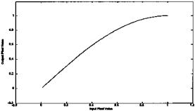
4.Load the image of a cancer cell (from rat prostate, courtesy of Alan W. Partin, M.D., Johns Hopkins University School of Medicine) cell.tif and apply a correction to the intensity values of the image (a gamma correction described in later chapters). Specifically, modify each pixel in the image by a

function that is a quarter wave sine wave. That is, the corrected pixels are the output of the sine function of the input pixels: Out(m,n) = f(In(m,n)) (see plot below).

FIGURE PROB. 10.4 Correction function to be used in Problem 4. The input pixel values are on the horizontal axis, and the output pixels values are on the vertical axis.

5.Load the blood cell image in blood1.tif. Write a sliding neighborhood function to enhance horizontal boundaries that go from dark to light. Write a second function that enhances boundaries that go from light to dark. Threshold both images so as to enhance the boundaries. Use a 3 by 2 sliding block. (Hint: This program may require several minutes to run. You do not need to rerun the program each time to adjust the threshold for the two binary images.)

6.Load the blood cells in blood.tif. Apply a distinct block function that replaces all of the values within a block by the maximum value in that block. Use a 4 by 4 block size. Repeat the operation using a function that replaces all the values by the minimum value in the block.

Copyright 2004 by Marcel Dekker, Inc. All Rights Reserved.

11

Image Processing:

Filters, Transformations,

and Registration

SPECTRAL ANALYSIS: THE FOURIER TRANSFORM

The Fourier transform and the efficient algorithm for computing it, the fast Fourier transform, extend in a straightforward manner to two (or more) dimensions. The two-dimensional version of the Fourier transform can be applied to images providing a spectral analysis of the image content. Of course, the resulting spectrum will be in two dimensions, and usually it is more difficult to interpret than a one-dimensional spectrum. Nonetheless, it can be a very useful analysis tool, both for describing the contents of an image and as an aid in the construction of imaging filters as described in the next section. When applied to images, the spatial directions are equivalent to the time variable in the onedimensional Fourier transform, and this analogous spatial frequency is given in terms of cycles/unit length (i.e., cycles/cm or cycles/inch) or normalized to cycles per sample. Many of the concerns raised with sampled time data apply to sampled spatial data. For example, undersampling an image will lead to aliasing. In such cases, the spatial frequency content of the original image is greater than fS/2, where fS now is 1/(pixel size). Figure 11.1 shows an example of aliasing in the frequency domain. The upper left-hand upper image contains a chirp signal increasing in spatial frequency from left to right. The high frequency elements on the right side of this image are adequately sampled in the left-hand image. The same pattern is shown in the upper right-hand image except that the sampling frequency has been reduced by a factor of 6. The right side of this image also contains sinusoidally varying intensities, but at additional frequencies as

Copyright 2004 by Marcel Dekker, Inc. All Rights Reserved.

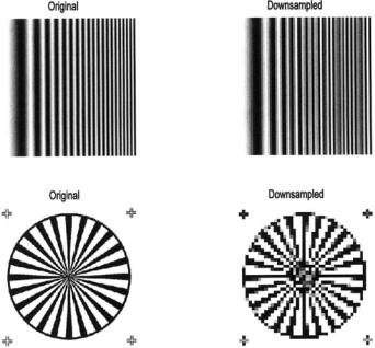
FIGURE 11.1 The influence of aliasing due to undersampling on two images with high spatial frequency. The aliased images show addition sinusoidal frequencies in the upper right image and jagged diagonals in the lower right image. (Lower original image from file ‘testpostl.png’ from the MATLAB Image Processing Toolbox. Copyright 1993–2003, The Math Works, Inc. Reprinted with permission.)

the aliasing folds other sinusoids on top of those in the original pattern. The lower figures show the influence of aliasing on a diagonal pattern. The jagged diagonals are characteristic of aliasing as are moire patterns seen in other images. The problem of determining an appropriate sampling size is even more acute in image acquisition since oversampling can quickly lead to excessive memory storage requirements.

The two-dimensional Fourier transform in continuous form is a direct extension of the equation given in Chapter 3:

m=−∞ n=−∞

The variables ω1 and ω2 are still frequency variables, although they define spatial frequencies and their units are in radians per sample. As with the time

Copyright 2004 by Marcel Dekker, Inc. All Rights Reserved.

domain spectrum, F(ω1,ω2) is a complex-valued function that is periodic in both ω1 and ω2. Usually only a single period of the spectral function is displayed, as was the case with the time domain analog.

The inverse two-dimensional Fourier transform is defined as:

As with the time domain equivalent, this statement is a reflection of the fact that any two-dimensional function can be represented by a series (possibly infinite) of sinusoids, but now the sinusoids extend over the two dimensions.

The discrete form of Eqs. (1) and (2) is again similar to their time domain analogs. For an image size of M by N, the discrete Fourier transform becomes:

The values F(p,q) are the Fourier Transform coefficients of f(m,n). The discrete form of the inverse Fourier Transform becomes:

MATLAB Implementation

Both the Fourier transform and inverse Fourier transform are supported in two (or more) dimensions by MATLAB functions. The two-dimensional Fourier transform is evoked as:

F = fft2(x,M,N);

where F is the output matrix and x is the input matrix. M and N are optional arguments that specify padding for the vertical and horizontal dimensions, respectively. In the time domain, the frequency spectrum of simple waveforms can usually be anticipated and the spectra of even relatively complicated waveforms can be readily understood. With two dimensions, it becomes more difficult to visualize the expected Fourier transform even of fairly simple images. In Example 11.1 a simple thin rectangular bar is constructed, and the Fourier transform of the object is constructed. The resultant spatial frequency function is plotted both as a three-dimensional function and as an intensity image.

Copyright 2004 by Marcel Dekker, Inc. All Rights Reserved.

Example 11.1 Determine and display the two-dimensional Fourier transform of a thin rectangular object. The object should be 2 by 10 pixels in size and solid white against a black background. Display the Fourier transform as both a function (i.e., as a mesh plot) and as an image plot.

%Example 11.1 Two-dimensional Fourier transform of a simple

%object.

%Construct a simple 2 by 10 pixel rectangular object, or bar.

%Take the Fourier transform padded to 256 by 256 and plot the

%result as a 3-dimensional function (using mesh) and as an

%intensity image.

%

%Construct object close all; clear all;

%Construct the rectangular object

%

imshow(f,’notruesize’); % Plot object

FIGURE 11.2A The rectangular object (2 pixels by 10 pixels used in Example 11.1. The Fourier transform of this image is shown in Figure 11.2B and C.

Copyright 2004 by Marcel Dekker, Inc. All Rights Reserved.

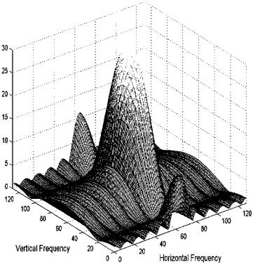
FIGURE 11.2B Fourier transform of the rectangular object in Figure 11.2A plotted as a function. More energy is seen, particularly at the higher frequencies, along the vertical axis because the object’s vertical cross sections appear as a narrow pulse. The border horizontal cross sections produce frequency characteristics that fall off rapidly at higher frequencies.

Note that in the above program the image size was kept small (22 by 30) since the image will be padded (with zeros, i.e., black) by ‘fft2.’ The fft2 routine places the DC component in the upper-left corner. The fftshift routine is used to shift this component to the center of the image for plotting purposes. The log of the function was taken before plotting as an image to improve the grayscale quality in the figure.

Copyright 2004 by Marcel Dekker, Inc. All Rights Reserved.

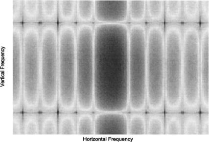
FIGURE 11.2C The Fourier transform of the rectangular object in Figure 11.2A plotted as an image. The log of the function was taken before plotting to improve the details. As in the function plot, more high frequency energy is seen in the vertical direction as indicated by the dark vertical band.

The horizontal chirp signal plotted in Figure 11.1 also produces a easily interpretable Fourier transform as shown in Figure 11.3. The fact that this image changes in only one direction, the horizontal direction, is reflected in the Fourier transform. The linear increase in spatial frequency in the horizontal direction produces an approximately constant spectral curve in that direction.

The two-dimensional Fourier transform is also useful in the construction and evaluation of linear filters as described in the following section.

LINEAR FILTERING

The techniques of linear filtering described in Chapter 4 can be directly extended to two dimensions and applied to images. In image processing, FIR filters are usually used because of their linear phase characteristics. Filtering an image is a local, or neighborhood, operation just as it was in signal filtering, although in this case the neighborhood extends in two directions around a given pixel. In image filtering, the value of a filtered pixel is determined from a linear combination of surrounding pixels. For the FIR filters described in Chapter 4,

Copyright 2004 by Marcel Dekker, Inc. All Rights Reserved.

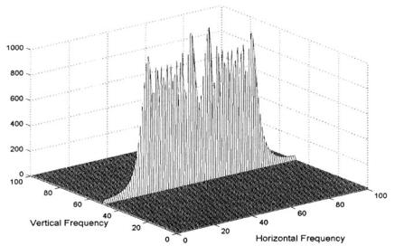
FIGURE 11.3 Fourier transform of the horizontal chirp signal shown in Figure 11.1. The spatial frequency characteristics of this image are zero in the vertical direction since the image is constant in this direction. The linear increase in spatial frequency in the horizontal direction is reflected in the more or less constant amplitude of the Fourier transform in this direction.

the linear combination for a given FIR filter was specified by the impulse response function, the filter coefficients, b(n). In image filtering, the filter function exists in two dimensions, h(m,n). These two-dimensional filter weights are applied to the image using convolution in an approach analogous to one-dimen- sional filtering.

The equation for two-dimensional convolution is a straightforward extension of the one-dimensional form (Eq. (15), Chapter 2):

k1=−∞ k2=−∞

While this equation would not be difficult to implement using MATLAB statements, MATLAB has a function that implements two-dimensional convolution directly.

Using convolution to perform image filtering parallels its use in signal imaging: the image array is convolved with a set of filter coefficients. However,

Copyright 2004 by Marcel Dekker, Inc. All Rights Reserved.

in image analysis, the filter coefficients are defined in two dimensions, h(m,n). A classic example of a digital image filter is the Sobel filter, a set of coefficients that perform a horizontal spatial derivative operation for enhancement of horizontal edges (or vertical edges if the coefficients are rotated using transposition):

These two-dimensional filter coefficients are sometimes referred to as the convolution kernel. An example of the application of a Sobel filter to an image is provided in Example 11.2.

When convolution is used to apply a series of weights to either image or signal data, the weights represent a two-dimensional impulse response, and, as with a one-dimensional impulse response, the weights are applied to the data in reverse order as indicated by the negative sign in the oneand two-dimensional convolution equations (Eq. (15) from Chapter 2 and Eq. (5).* This can become a source of confusion in two-dimensional applications. Image filtering is easier to conceptualize if the weights are applied directly to the image data in the same orientation. This is possible if digital filtering is implemented using correlation rather that convolution. Image filtering using correlation is a sliding neighborhood operation, where the value of the center pixel is just the weighted sum of neighboring pixels with the weighting given by the filter coefficients. When correlation is used, the set of weighting coefficients is termed the correlation kernel to distinguish it from the standard filter coefficients. In fact, the operations of correlation and convolution both involve weighted sums of neighboring pixels, and the only difference between correlation kernels and convolution kernels is a 180-degree rotation of the coefficient matrix. MATLAB filter routines use correlation kernels because their application is easier to conceptualize.

MATLAB Implementation

Two dimensional-convolution is implemented using the routine ‘conv2’:

I2 = conv2(I1, h, shape)

where I1 and h are image and filter coefficients (or two images, or simply two matrices) to be convolved and shape is an optional argument that controls the size of the output image. If shape is ‘full’, the default, then the size of the output matrix follows the same rules as in one-dimensional convolution: each

*In one dimension, this is equivalent to applying the weights in reverse order. In two dimensions, this is equivalent to rotating the filter matrix by 180 degrees before multiplying corresponding pixels and coefficients.

Copyright 2004 by Marcel Dekker, Inc. All Rights Reserved.