Biosignal and Biomedical Image Processing MATLAB based Applications - John L. Semmlow

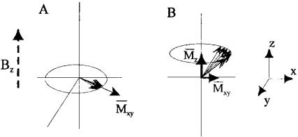
cal property known as spin.* In MRI lingo, the nucleus and/or the associated magnetic dipole is termed a spin. For clinical imaging, the hydrogen proton is used because it occurs in large numbers in biological tissue. Although there are a large number of hydrogen protons, or spins, in biological tissue (1 mm3 of water contains 6.7 × 1019 protons), the net magnetic moment that can be produced, even if they were all aligned, is small due to the near balance between spin-up (1⁄2) and spin-down (−1⁄2) states. When they are placed in a magnetic field, the magnetic dipoles are not static, but rotate around the axis of the applied magnetic field like spinning tops, Figure 13.11A (hence, the spins themselves spin). A group of these spins produces a net moment in the direction of the magnetic field, z, but since they are not in phase, any horizontal moment in the x and y direction tends to cancel (Figure 13.11B).

While the various spins do not have the same relative phase, they do all rotate at the same frequency, a frequency given by the Larmor equation:

FIGURE 13.11 (A) A single proton has a magnetic moment which rotates in the presence of an applied magnet field, Bz. This dipole moment could be up or down with a slight favoritism towards up, as shown. (B) A group of upward dipoles create a net moment in the same direction as the magnetic field, but any horizontal moments (x or y) tend to cancel. Note that all of these dipole vectors should be rotating, but for obvious reasons they are shown as stationary with the assumption that they rotate, or more rigorously, that the coordinate system is rotating.

*Nuclear spin is not really a spin, but another one of those mysterious quantum mechanical properties. Nuclear spin can take on values of ±1/2, with +1/2 slightly favored in a magnetic field.

Copyright 2004 by Marcel Dekker, Inc. All Rights Reserved.

where ωo is the frequency in radians, H is the magnitude of the magnitude field, and γ is a constant termed the gyromagnetic constant. Although γ is primarily a function of the type of nucleus it also depends slightly on the local chemical environment. As shown below, this equation contains the key to spatial localization in MRI: variations in local magnetic field will encode as variations in rotational frequency of the protons.

If these rotating spins are exposed to electromagnetic energy at the rotational or Larmor frequency specified in Eq. (11), they will absorb this energy and rotate further and further from their equilibrium position near the z axis: they are tipped away from the z axis (Figure 13.12A). They will also be synchronized by this energy, so that they now have a net horizontal moment. For protons, the Larmor frequency is in the radio frequency (rf ) range, so an rf pulse of the appropriate frequency in the xy-plane will tip the spins away from the z-axis an amount that depends on the length of the pulse:

where θ is the tip angle and Tp pulse time. Usually Tp is adjusted to tip the angle either 90 or 180 deg. As described subsequently, a 90 deg. tip is used to generate the strongest possible signal and an 180 deg tip, which changes the sign of the

FIGURE 13.12 (A) After an rf pulse that tips the spins 90 deg., the net magnetic moment looks like a vector, Mxy, rotating in the xy-plane. The net vector in the z direction is zero. (B) After the rf energy is removed, all of the spins begin to relax back to their equilibrium position, increasing the z component, Mz, and decreasing the xy component, Mxy. The xy component also decreases as the spins desynchronize.

Copyright 2004 by Marcel Dekker, Inc. All Rights Reserved.

moment, is used to generate an echo signal. Note that a given 90 or 180 deg. Tp will only flip those spins that are exposed to the appropriate local magnetic field, H.

When all of the spins in a region are tipped 90 deg. and synchronized, there will be a net magnetic moment rotating in the xy-plane, but the component of the moment in the z direction will be zero (Figure 13.12A). When the rf pulse ends, the rotating magnetic field will generate its own rf signal, also at the Larmor frequency. This signal is known as the free induction decay (FID) signal. It is this signal that induces a small voltage in the receiver coil, and it is this signal that is used to construct the MR image. Immediately after the pulse ends, the signal generated is given by:

where ωo is the Larmor frequency, θ is the tip angle, and ρ is the density of spins. Note that a tip angle of 90 deg. produces the strongest signal.

Over time the spins will tend to relax towards the equilibrium position (Figure 13.12B). This relaxation is known as the longitudinal or spin-lattice relaxation time and is approximately exponential with a time constant denoted as “T1.” As seen in Figure 13.12B, it has the effect of increasing the horizontal moment, Mz, and decreasing the xy moment, Mxy. The xy moment is decreased even further, and much faster, by a loss of synchronization of the collective spins, since they are all exposed to a slightly different magnetic environment from neighboring atoms (Figure 13.12B). This so-called transverse or spin-spin relaxation time is also exponential and decays with a time constant termed “T2.” The spin-spin relaxation time is always less than the spin lattice relaxation time, so that by the time the net moment returns to equilibrium position along the z axis the individual spins are completely de-phased. Local inhomogeneities in the applied magnetic field cause an even faster de-phasing of the spins. When

the de-phasing time constant is modified to include this effect, it is termed T *

2

(pronounced tee two star). This time constant also includes the T2 influences. When these relaxation processes are included, the equation for the FID signals becomes:

While frequency dependence (i.e., the Larmor equation) is used to achieve localization, the various relation times as well as proton density are used to achieve image contrast. Proton density, ρ, for any given collection of spins is a relatively straightforward measurement: it is proportional to FID signal ampli-

tude as shown in Eq. (14). Measuring the local T and T (or T *) relaxation

1 2 2

times is more complicated and is done through clever manipulations of the rf pulse and local magnetic field gradients, as briefly described in the next section.

Copyright 2004 by Marcel Dekker, Inc. All Rights Reserved.

Data Acquisition: Pulse Sequences

A combination of rf pulses, magnetic gradient pulses, delays, and data acquisition periods is termed a pulse sequence. One of the clever manipulations used in many pulse sequences is the spin echo technique, a trick for eliminating the de-phasing caused by local magnetic field inhomogeneities and related artifacts

(the T * decay). One possibility might be to sample immediately after the rf

2

pulse ends, but this is not practical. The alternative is to sample a realigned echo. After the spins have begun to spread out, if their direction is suddenly reversed they will come together again after a known delay. The classic example is that of a group of runners who are told to reverse direction at the same time, say one minute after the start. In principal, they all should get back to the start line at the same time (one minute after reversing) since the fastest runners will have the farthest to go at the time of reversal. In MRI, the reversal is accomplished by a phase-reversing 180 rf pulse. The realignment will occur with the

same time constant, T *, as the misalignment. This echo approach will only

2

cancel the de-phasing due to magnetic inhomogeneities, not the variations due to the sample itself: i.e., those that produce the T2 relaxation. That is actually desirable because the sample variations that cause T2 relaxation are often of interest.

As mentioned above, the Larmor equation (Eq. (11)) is the key to localization. If each position in the sample is subjected to a different magnetic field strength, then the locations are tagged by their resonant frequencies. Two approaches could be used to identify the signal from a particular region. Use an rf pulse with only one frequency component, and if each location has a unique magnetic field strength then only the spins in one region will be excited, those whose magnetic field correlates with the rf frequency (by the Larmor equation). Alternatively excite a broader region, then vary the magnetic field strength so that different regions are given different resonant frequencies. In clinical MRI, both approaches are used.

Magnetic field strength is varied by the application of gradient fields applied by electromagnets, so-called gradient coils, in the three dimensions. The gradient fields provide a linear change in magnetic field strength over a limited area within the MR imager. The gradient field in the z direction, Gz, can be used to isolate a specific xy slice in the object, a process known as slice selection.* In the absence of any other gradients, the application of a linear gradient in the z direction will mean that only the spins in one xy-plane will have a resonant frequency that matches a specific rf pulse frequency. Hence, by adjusting the

*Selected slices can be in any plane, x, y, z, or any combination, by appropriate activation of the gradients during the rf pulse. For simplicity, this discussion assumes the slice is selected by the z- gradient so spins in an xy-plane are excited.

Copyright 2004 by Marcel Dekker, Inc. All Rights Reserved.

gradient, different xy-slices will be associated with (by the Larmor equation), and excited by, a specific rf frequency. Since the rf pulse is of finite duration it cannot consist of a single frequency, but rather has a range of frequencies, i.e., a finite bandwidth. The thickness of the slice, that is, the region in the z-direc- tion over which the spins are excited, will depend on the steepness of the gradient field and the bandwidth of the rf pulse:

Very thin slices, ∆z, would require a very narrowband pulse, ∆ω, in combination with a steep gradient field, Gz.

If all three gradients, Gx, Gy, and Gz, were activated prior to the rf pulse then only the spins in one unique volume would be excited. However, only one data point would be acquired for each pulse repetition, and to acquire a large volume would be quite time-consuming. Other strategies allow the acquisition of entire lines, planes, or even volumes with one pulse excitation. One popular pulse sequence, the spin-echo pulse sequence, acquires one line of data in the spatial frequency domain. The sequence begins with a shaped rf pulse in conjunction with a Gz pulse that provides slice selection (Figure 13.13). The Gz includes a reversal at the end to cancel a z-dependent phase shift. Next, a y- gradient pulse of a given amplitude is used to phase encode the data. This is followed by a second rf/Gz combination to produce the echo. As the echo regroups the spins, an x-gradient pulse frequency encodes the signal. The reformed signal constitutes one line in the ferquency domain (termed k-space in MRI), and is sampled over this period. Since the echo signal duration is several hundred microseconds, high-speed data acquisition is necessary to sample up to 256 points during this signal period.

As with slice thickness, the ultimate pixel size will depend on the strength of the magnetic gradients. Pixel size is directly related to the number of pixels in the reconstructed image and the actual size of the imaged area, the so-called field-of-view (FOV). Most modern imagers are capable of a 2 cm FOV with samples up to 256 by 256 pixels, giving a pixel size of 0.078 mm. In practice, image resolution is usually limited by signal-to-noise considerations since, as pixel area decreases, the number of spins available to generate a signal diminishes proportionately. In some circumstances special receiver coils can be used to increase the signal-to-noise ratio and improve image quality and/or resolution. Figure 13.14A shows an image of the Shepp-Logan phantom and the same image acquired with different levels of detector noise.* As with other forms of signal processing, MR image noise can be improved by averaging. Figure

*The Shepp-Logan phantom was developed to demonstrate the difficulty of identifying a tumor in a medical image.

Copyright 2004 by Marcel Dekker, Inc. All Rights Reserved.

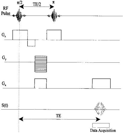
FIGURE 13.13 The spin-echo pulse sequence. Events are timed with respect to the initial rf pulse. See text for explanation.

13.14D shows the noise reduction resulting from averaging four of the images taken under the same noise conditions as Figure 13.14C. Unfortunately, this strategy increases scan time in direct proportion to the number of images averaged.

Functional Magnetic Resonance Imaging

Image processing for MR images is generally the same as that used on other images. In fact, MR images have been used in a number of examples and problems in previous chapters. One application of MRI does have some unique im-

Copyright 2004 by Marcel Dekker, Inc. All Rights Reserved.

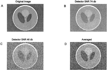
FIGURE 13.14 (A) MRI reconstruction of a Shepp-Logan phantom. (B) and (C) Reconstruction of the phantom with detector noise added to the frequency domain signal. (D) Frequency domain average of four images taken with noise similar to C. Improvement in the image is apparent. (Original image from the MATLAB Image Processing Toolbox. Copyright 1993–2003, The Math Works, Inc. Reprinted with permission.)

age processing requirements: the area of functional magnetic resonance imaging (fMRI). In this approach, neural areas that are active in specific tasks are identified by increases in local blood flow. MRI can detect cerebral blood changes using an approach known as BOLD: blood oxygenation level dependent. Special pulse sequences have been developed that can acquire images very quickly, and these images are sensitive to the BOLD phenomenon. However, the effect is very small: changes in signal level are only a few percent.

During a typical fMRI experiment, the subject is given a task which is either physical (such a finger tapping), purely sensory (such as a flashing visual stimulus), purely mental (such as performing mathematical calculations), or involves sensorimotor activity (such as pushing a button whenever a given image appears). In single-task protocols, the task alternates with non-task or baseline activity period. Task periods are usually 20–30 seconds long, but can be shorter and can even be single events under certain protocols. Multiple task protocols are possible and increasingly popular. During each task a number of MR images

Copyright 2004 by Marcel Dekker, Inc. All Rights Reserved.

are acquired. The primary role of the analysis software is to identify pixels that have some relationship to the task/non-task activity.

There are a number of software packages available that perform fMRI analysis, some written in MATLAB such as SPM, (statistical parametric mapping), others in c-language such as AFNI (analysis of neural images). Some packages can be obtained at no charge off the Web. In addition to identifying the active pixels, these packages perform various preprocessing functions such as aligning the sequential images and reshaping the images to conform to standard models of the brain.

Following preprocessing, there are a number of different approaches to identifying regions where local blood flow correlates with the task/non-task timing. One approach is simply to use correlation, that is correlate the change in signal level, on a pixel-by-pixel basis, with a task-related function. This function could represent the task by a one and the non-task by a zero, producing a square wave-like function. More complicated task functions account for the dynamics of the BOLD process which has a 4 to 6 second time constant. Finally, some new approaches based on independent component analysis (ICA, Chapter 9) can be used to extract the task function from the data itself. The use of correlation and ICA analysis is explored in the MATLAB Implementation section and in the problems. Other univariate statistical techniques are common such as t-tests and f-tests, particularly in the multi-task protocols (Friston, 2002).

MATLAB Implementation

Techniques for fMRI analysis can be implemented using standard MATLAB routines. The identification of active pixels using correlation with a task protocol function will be presented in Example 13.4. Several files have been created on the disk that simulate regions of activity in the brain. The variations in pixel intensity are small, and noise and other artifacts have been added to the image data, as would be the case with real data. The analysis presented here is done on each pixel independently. In most fMRI analyses, the identification procedure might require activity in a number of adjoining pixels for identification. Lowpass filtering can also be used to smooth the image.

Example 13.4 Use correlation to identify potentially active areas from MRI images of the brain. In this experiment, 24 frames were taken (typical fMRI experiments would contain at least twice that number): the first 6 frames were acquired during baseline activity and the next 6 during the task. This offon cycle was then repeated for the next 12 frames. Load the image in MATLAB file fmril, which contains all 24 frames. Generate a function that represents the off-on task protocol and correlate this function with each pixel’s variation over the 24 frames. Identify pixels that have correlation above a given threshold and mark the image where these pixels occur. (Usually this would be done in color with higher correlations given brighter color.) Finally display the time sequence

Copyright 2004 by Marcel Dekker, Inc. All Rights Reserved.

of one of the active pixels. (Most fMRI analysis packages can display the time variation of pixels or regions, usually selected interactively.)

%Example 13.4 Example of identification of active area

%using correlation.

%Load the 24 frames of the image stored in fmri1.mat.

%Construct a stimulus profile.

%In this fMRI experiment the first 6 frames were taken during

%no-task conditions, the next six frames during the task

%condition, and this cycle was repeated.

%Correlate each pixel’s variation over the 24 frames with the

%task profile. Pixels that correlate above a certain threshold

%(use 0.5) should be identified in the image by a pixel

%whose intensity is the same as the correlation values

%

clear all; close all thresh = .5;

load fmri1;

i_stim2 = ones(24,1); i_stim2(1:6) = 0; i_stim2(13:18) = 0;

%

% Do correlation: pixel by pixel over the 24 frames I_fmri_marked = I_fmri;

active = [0 0]; for i = 1:128

for j = 1:128 for k = 1:24

temp(k) = I_fmri(i,j,1,k);

end

cor_temp = corrcoef([temp’i_stim2]);

corr(i,j) = cor_temp(2,1); % Get correlation value if corr(i,j) > thresh

end end

end

%

% Display marked image imshow(I_fmri_marked(:,:,:,1)); title(‘fMRI Image’); figure;

% Display one of the active areas

for i = 1:24 % Plot one of the active areas

Copyright 2004 by Marcel Dekker, Inc. All Rights Reserved.

active_neuron(i) = I_fmri(active(2,1),active(2,2),:,i); end

plot(active_neuron); title(‘Active neuron’);

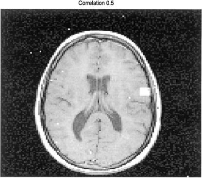
The marked image produced by this program is shown in Figure 13.15. The actual active area is the rectangular area on the right side of the image slightly above the centerline. However, a number of other error pixels are present due to noise that happens to have a sufficiently high correlation with the task profile (a correlation of 0.5 in this case). In Figure 13.16, the correlation threshold has been increased to 0.7 and most of the error pixels have been

FIGURE 13.15 White pixels were identified as active based on correlation with the task profile. The actual active area is the rectangle on the right side slightly above the center line. Due to inherent noise, false pixels are also identified, some even outside of the brain. The correlation threshold was set a 0.5 for this image. (Original image from the MATLAB Image Processing Toolbox. Copyright 1993– 2003, The Math Works, Inc. Reprinted with permission.)

Copyright 2004 by Marcel Dekker, Inc. All Rights Reserved.