Biosignal and Biomedical Image Processing MATLAB based Applications - John L. Semmlow

FIGURE 12.14 Image of cells (left) on a gray background. The textural image (right) was created based on local variance (standard deviation) and shows somewhat more definition. (Cancer cell from rat prostate, courtesy of Alan W. Partin, M.D., Ph.D., Johns Hopkins University School of Medicine.)

Copyright 2004 by Marcel Dekker, Inc. All Rights Reserved.

FIGURE 12.15 Isolated portions of the cells shown in Figure 12.14. The upper images were created by thresholding the intensity. The lower left image is a combination (logical OR) of the upper images and the lower right image adds a thresholded texture-based image.

The original and texture images are shown in Figure 12.14. Note that the texture image has been scaled up, first by a factor of six, then by an additional factor of two, to bring it within a nominal image range. The intensity thresholded images are shown in Figure 12.15 (upper images; the upper right image has been inverted). These images are combined in the lower left image. The lower right image shows the combination of both intensity-based images with the thresholded texture image. This method of combining images can be extended to any number of different segmentation approaches.

MORPHOLOGICAL OPERATIONS

Morphological operations have to do with processing shapes. In this sense they are continuity-based techniques, but in some applications they also operate on

Copyright 2004 by Marcel Dekker, Inc. All Rights Reserved.

edges, making them useful in edge-based approaches as well. In fact, morphological operations have many image processing applications in addition to segmentation, and they are well represented and supported in the MATLAB Image Processing Toolbox.

The two most common morphological operations are dilation and erosion. In dilation the rich get richer and in erosion the poor get poorer. Specifically, in dilation, the center or active pixel is set to the maximum of its neighbors, and in erosion it is set to the minimum of its neighbors. Since these operations are often performed on binary images, dilation tends to expand edges, borders, or regions, while erosion tends to decrease or even eliminate small regions. Obviously, the size and shape of the neighborhood used will have a very strong influence on the effect produced by either operation.

The two processes can be done in tandem, over the same area. Since both erosion and dilation are nonlinear operations, they are not invertible transformations; that is, one followed by the other will not generally result in the original image. If erosion is followed by dilation, the operation is termed opening. If the image is binary, this combined operation will tend to remove small objects without changing the shape and size of larger objects. Basically, the initial erosion tends to reduce all objects, but some of the smaller objects will disappear altogether. The subsequent dilation will restore those objects that were not eliminated by erosion. If the order is reversed and dilation is performed first followed by erosion, the combined process is called closing. Closing connects objects that are close to each other, tends to fill up small holes, and smooths an object’s outline by filling small gaps. As with the more fundamental operations of dilation and erosion, the size of objects removed by opening or filled by closing depends on the size and shape of the neighborhood that is selected.

An example of the opening operation is shown in Figure 12.16 including the erosion and dilation steps. This is applied to the blood cell image after thresholding, the same image shown in Figure 12.3 (left side). Since we wish to eliminate black artifacts in the background, we first invert the image as shown in Figure 12.16. As can be seen in the final, opened image, there is a reduction in the number of artifacts seen in the background, but there is also now a gap created in one of the cell walls. The opening operation would be more effective on the image in which intermediate values were masked out (Figure 12.3, right side), and this is given as a problem at the end of the chapter.

Figure 12.17 shows an example of closing applied to the same blood cell image. Again the operation was performed on the inverted image. This operation tends to fill the gaps in the center of the cells; but it also has filled in gaps between the cells. A much more effective approach to filling holes is to use the imfill routine described in the section on MATLAB implementation.

Other MATLAB morphological routines provide local maxima and minima, and allows for manipulating the image’s maxima and minima, which implement various fill-in effects.

Copyright 2004 by Marcel Dekker, Inc. All Rights Reserved.

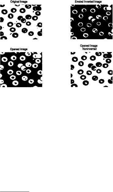
FIGURE 12.16 Example of the opening operation to remove small artifacts. Note that the final image has fewer background spots, but now one of the cells has a gap in the wall.

MATLAB Implementation

The erosion and dilation could be implemented using the nonlinear filter routine nlfilter, although this routine limits the shape of the neighborhood to a rectangle. The MATLAB routines imdilate and imerode provide for a variety of neighborhood shapes and are much faster than nlfilter. As mentioned above, opening consists of erosion followed by dilation and closing is the reverse. MATLAB also provide routines for implementing these two operations in one statement.

To specify the neighborhood used by all of these routines, MATLAB uses a structuring element.* A structuring element can be defined by a binary array, where the ones represent the neighborhood and the zeros are irrelevant. This allows for easy specification of neighborhoods that are nonrectangular, indeed that can have any arbitrary shape. In addition, MATLAB makes a number of popular shapes directly available, just as the fspecial routine makes a number

*Not to be confused with a similar term, structural unit, used in the beginning of this chapter. A structural unit is the object of interest in the image.

Copyright 2004 by Marcel Dekker, Inc. All Rights Reserved.

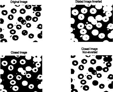
FIGURE 12.17 Example of closing to fill gaps. In the closed image, some of the cells are now filled, but some of the gaps between cells have been erroneously filled in.

of popular two-dimensional filter functions available. The routine to specify the structuring element is strel and is called as:

structure = strel(shape, NH, arg);

where shape is the type of shape desired, NH usually specifies the size of the neighborhood, and arg and an argument, frequently optional, that depends on shape. If shape is ‘arbitrary’, or simply omitted, then NH is an array that specifies the neighborhood in terms of ones as described above. Prepackaged shapes include:

Copyright 2004 by Marcel Dekker, Inc. All Rights Reserved.

For many of these shapes, the routine strel produces a decomposed structure that runs significantly faster.

Based on the structure, the statements for dilation, erosion, opening, and closing are:

I1 = imdilate(I, structure);

I1 = imerode(I, structure);

I1 = imopen(I, structuure);

I1 = imclose(I, structure);

where I1 is the output image, I is the input image and structure is the neighborhood specification given by strel, as described above. In all cases, structure can be replaced by an array specifying the neighborhood as ones, bypassing the strel routine. In addition, imdilate and imerode have optional arguments that provide packing and unpacking of the binary input or output images.

Example 12.5 Apply opening and closing to the thresholded blood cell images of Figure 12–3 in an effort to remove small background artifacts and to fill holes. Use a circular structure with a diameter of four pixels.

%Example 12.5 and Figures 12.16 and 12.17

%Demonstration of morphological opening to eliminate small

%artifacts and of morphological closing to fill gaps

%These operations will be applied to the thresholded blood cell

%images of Figure 12.3 (left image).

%Uses a circular or disk shaped structure 4 pixels in diameter

clear all; close all;

I = imread(‘blood1.tif’);

I = im2double(I);

BW = im2bw(I,thresh(I));

%

SE = strel(‘disk’,4);

BW1= imerode(BW,SE);

BW2 = imdilate(BW1,SE);

%

.......display images.....

%

.......display images.....

Copyright 2004 by Marcel Dekker, Inc. All Rights Reserved.

This example produced the images in Figures 12.15 and 12.16.

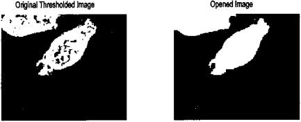
Example 12.6 Apply an opening operation to remove the dark patches seen in the thresholded cell image of Figure 12.15.

%Figures 12.6 and 12.18

%Use opening to remove the dark patches in the thresholded cell

%image of Figure 12.15

%

close all; clear all;

%

SE = strel(‘square’,5);

load fig12_15;

BW1= imopen( BW2,SE);

.......Display images.....

The result of this operation is shown in Figure 12.18. In this case, the closing operation is able to remove completely the dark patches in the center of the cell image. A 5-by-5 pixel square structural element was used. The size (and shape) of the structural element controlled the size of artifact removed, and no attempt was made to optimize its shape. The size was set here as the minimum that would still remove all of the dark patches. The opening operation in this example used the single statement imopen. Again, the opening operation operates on activated (i.e., white pixels), so to remove dark artifacts it is necessary to invert the image (using the logical NOT operator, ) before performing the opening operation. The opened image is then inverted again before display.

FIGURE 12.18 Application of the open operation to remove the dark patches in the binary cell image in Figure 12.15 (lower right). Using a 5 by 5 square structural element resulted in eliminating all of the dark patches.

Copyright 2004 by Marcel Dekker, Inc. All Rights Reserved.

MATLAB morphology routines also allow for manipulation of maxima and minima in an image. This is useful for identifying objects, and for filling. Of the many other morphological operations supported by MATLAB, only the imfill operation will be described here. This operation begins at a designated pixel and changes connected background pixels (0’s) to foreground pixels (1’s), stopping only when a boundary is reached. For grayscale images, imfill brings the intensity levels of the dark areas that are surrounded by lighter areas up to the same intensity level as surrounding pixels. (In effect, imfill removes regional minima that are not connected to the image border.) The initial pixel can be supplied to the routine or obtained interactively. Connectivity can be defined as either four connected or eight connected. In four connectivity, only the four pixels bordering the four edges of the pixel are considered, while in eight connectivity all pixel that touch, including those that touch only at the corners, are considered connected.

The basic imfill statement is:

I_out = imfill(I, [r c], con);

where I is the input image, I_out is the output image, [r c] is a two-element vector specifying the beginning point, and con is an optional argument that is set to 8 for eight connectivity (four connectivity is the default). (See the help file to use imfill interactively.) A special option of imfill is available specifically for filling holes. If the image is binary, a hole is a set of background pixels that cannot be reached by filling in the background from the edge of the image. If the image is an intensity image, a hole is an area of dark pixels surrounded by lighter pixels. To invoke this option, the argument following the input image should be holes. Figure 12.19 shows the operation performed on the blood cell image by the statement:

I_out = imfill(I, ‘holes’);

EDGE-BASED SEGMENTATION

Historically, edge-based methods were the first set of tools developed for segmentation. To move from edges to segments, it is necessary to group edges into chains that correspond to the sides of structural units, i.e., the structural boundaries. Approaches vary in how much prior information they use, that is, how much is used of what is known about the possible shape. False edges and missed edges are two of the more obvious, and more common, problems associated with this approach.

The first step in edge-based methods is to identify edges which then become candidates for boundaries. Some of the filters presented in Chapter 11

Copyright 2004 by Marcel Dekker, Inc. All Rights Reserved.

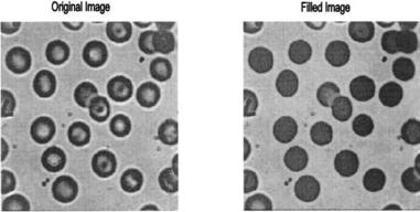
FIGURE 12.19 Hole filling operation produced by imfill. Note that neither the edge cell (at the upper image boundary) or the overlapped cell in the center are filled since they are not actually holes. (Original image reprinted with permission from the Image Processing Handbook 2nd edition. Copyright CRC Press, Boca Raton, Florida.)

perform edge enhancement, including the Sobel, Prewitt, and Log filters. In addition, the Laplacian, which takes the spatial second derivative, can be used to find edge candidates. The Canny filter is the most advanced edge detector supported by MATLAB, but it necessarily produces a binary output while many of the secondary operations require a graded edge image.

Edge relaxation is one approach used to build chains from individual edge candidate pixels. This approach takes into account the local neighborhood: weak edges positioned between strong edges are probably part of the edge, while strong edges in isolation are likely spurious. The Canny filter incorporates a type of edge relaxation. Various formal schemes have been devised under this category. A useful method is described in Sonka (1995) that establishes edges between pixels (so-called crack edges) based on the pixels located at the end points of the edge.

Another method for extending edges into chains is termed graph searching. In this approach, the endpoints (which could both be the same point in a closed boundary) are specified, and the edge is determined based on minimizing some cost function. Possible pathways between the endpoints are selected from candidate pixels, those that exceed some threshold. The actual path is selected based on a minimization of the cost function. The cost function could include features such as the strength of an edge pixel and total length, curvature, and proximity of the edge to other candidate borders. This approach allows for a

Copyright 2004 by Marcel Dekker, Inc. All Rights Reserved.

great deal of flexibility. Finally, dynamic programming can be used which is also based on minimizing a cost function.

The methods briefly described above use local information to build up the boundaries of the structural elements. Details of these methods can be found in Sonka et al. (1995). Model-based edge detection methods can be used to exploit prior knowledge of the structural unit. For example, if the shape and size of the image is known, then a simple matching approach based on correlation can be used (matched filtering). When the general shape is known, but not the size, the Hough transform can be used. This approach was originally designed for identifying straight lines and curves, but can be expanded to other shapes provided the shape can be described analytically.

The basic idea behind the Hough transform is to transform the image into a parameter space that is constructed specifically to describe the desired shape analytically. Maxima in this parameter space then correspond to the presence of the desired image in image space. For example, if the desired object is a straight line (the original application of the Hough transform), one analytic representation for this shape is y = mx + b,* and such shapes can be completely defined by a two-dimensional parameter space of m and b parameters. All straight lines in image space map to points in parameter space (also known as the accumulator array for reasons that will become obvious). Operating on a binary image of edge pixels, all possible lines through a given pixel are transformed into m,b combinations, which then increment the accumulator array. Hence, the accumulator array accumulates the number of potential lines that could exist in the image. Any active pixel will give rise to a large number of possible line slopes, m, but only a limited number of m,b combinations. If the image actually contains a line, then the accumulator element that corresponds to that particular line’s m,b parameters will have accumulated a large number. The accumulator array is searched for maxima, or supra threshold locations, and these locations identify a line or lines in the image.

This concept can be generalized to any shape that can be described analytically, although the parameter space (i.e., the accumulator) may have to include several dimensions. For example, to search for circles note that a circle can be defined in terms of three parameters, a, s, and r for the equation given below.

where a and b define the center point of the circle and r is the radius. Hence the accumulator space must be three-dimensional to represent a, b, and r.

*This representation of a line will not be able to represent vertical lines since m → ∞ for a vertical line. However, lines can also be represented in two dimensions using cylindrical coordinates, r and θ: y = r cos θ + r sin θ.

Copyright 2004 by Marcel Dekker, Inc. All Rights Reserved.