Biosignal and Biomedical Image Processing MATLAB based Applications - John L. Semmlow

where name is the name of the specific window function (preceded by @), N the number of points desired, and opt possible optional argument(s) required by some specific windows.

To apply a window to the Fourier series analysis such as in Example 2.1, simply point-by-point multiply the digitized waveform by the output of the MATLAB window_name routine before calling the FFT routine. For example:

Note that in the example above it was necessary to transpose the window function W so that it was in the same format as the data. The window function produces a row vector.

Figure 3.12 shows two spectra obtained from a data set consisting of two sine waves closely spaced in frequency (235 Hz and 250 Hz) with added white noise in a 256 point array sampled at 1 kHz. Both spectra used the Welch method with the same parameters except for the windowing. (The window func-

FIGURE 3.12 Two spectra computed for a waveform consisting of two closely spaced sine waves (235 and 250 Hz) in noise (SNR = −10 db). Welch’s method was used for both methods with the same parameters (nfft = 128, overlap = 64) except for the window functions.

Copyright 2004 by Marcel Dekker, Inc. All Rights Reserved.

tion can be embedded in the pwelch calling structure.) The upper spectrum was obtained using a Hamming window (hamming) which has large sidelobes, but a fairly narrow mainlobe while the lower spectrum used a Chebyshev window (chebwin) which has small sidelobes but a larger mainlobe.

A small difference is seen in the ability to resolve the two peaks. The Hamming window with a smaller main lobe gives rise to a spectrum that shows two peaks while the presence of two peaks might be missed in the Chebyshev windowed spectrum.

PROBLEMS

1.(A) Construct two arrays of white noise: one 128 points in length and the other 1024 points in length. Take the FT of both. Does increasing the length improve the spectral estimate of white noise?

(B) Apply the Welch methods to the longer noise array using a Hanning window with an nfft of 128 with no overlap. Does this approach improve the spectral estimate? Now change the overlap to 64 and note any changes in the spectrum. Submit all frequency plots appropriately labeled.

2.Find the power spectrum of the filtered noise data from Problem 3 in Chap- ter 2 using the standard FFT. Show frequency plots appropriately labeled. Scale, or rescale, the frequency axis to adequately show the frequency response of this filter.

3.Find the power spectrum of the filtered noise data in Problem 2 above using the FFT, but zero pad the data so that N = 2048. Note the visual improvement in resolution.

4.Repeat Problem 2 above using the data from Problem 6 in Chapter 2. Applying the Hamming widow to the data before calculating the FFT.

5.Repeat problem 4 above using the Welch method with 256 and 65 segment lengths and the window of your choice.

6.Repeat Problem 4 above using the data from Problem 7, Chapter 2.

7.Use routine sig_noise noise to generate a 256-point array that contains two closely spaced sinusoids at 140 and 180 Hz both with an SNR of -10 db. (Calling structure: data = sig_noise([140 180], [-10 -10], 256);) Sig_noise assumes a sampling rate of 1 kHz. Use the Welch method. Find the

spectrum of the waveform for segment lengths of 256 (no overlap) and 64 points with 0%, 50% and 99% overlap.

8. Use sig_noise to generate a 512-point array that contains a single sinusoid at 200 Hz with an SNR of -12 db. Find the power spectrum first by taking the

Copyright 2004 by Marcel Dekker, Inc. All Rights Reserved.

FFT of the autocorrelation function. Compare this power spectrum with the one obtained using the direct method. Plot the two spectra side-by-side.

9.Using the data of Problem 7 above, find the power spectrum applying the Welch method with 64-point segments, and no overlap. Using the Chebyshev (chebwin), Kaiser (kaiser), and Gauss (gausswin) windows, find the best window in terms of frequency separation. Submit frequency plots obtained using the best and worse windows (in terms of separation). For the Chebyshev window use a ripple of 40 db, and for the Kaiser window use a beta of 0 (minimum mainlobe option).

10.Use routine sig_noise to generate a 512-point array containing one sinusoid at 150 Hz and white noise; SNR = −15db. Generate the power spectrum as the square of the magnitude obtained using the Fourier transform. Put the signal generator commands and spectral analysis commands in a loop and calculate the spectrum five times plotting the five spectra superimposed. Repeat using the Welch method and data segment length of 128 and a 90% overlap.

Copyright 2004 by Marcel Dekker, Inc. All Rights Reserved.

4

Digital Filters

Filters are closely related to spectral analysis since the goal of filtering is to reshape the spectrum to one’s advantage. Most noise is broadband (the broadestband noise being white noise with a flat spectrum) and most signals are narrowband; hence, filters that appropriately reshape a waveform’s spectrum will almost always provide some improvement in SNR. As a general concept, a basic filter can be viewed as a linear process in which the input signal’s spectrum is reshaped in some well-defined (and, one hopes, beneficial) manner. Filters differ in the way they achieve this spectral reshaping, and can be classified into two groups based on their approach. These two groups are termed finite impulse response (FIR) filters and infinite impulse response (IIR) filters, although this terminology is based on characteristics which are secondary to the actual methodology. We will describe these two approaches separately, clarifying the major differences between them. As in preceding chapters, these descriptions will be followed by a presentation of the MATLAB implementation.

THE Z-TRANSFORM

The frequency-based analysis introduced in the last chapter is a most useful tool for analyzing systems or responses in which the waveforms are periodic or aperiodic, but cannot be applied to transient responses of infinite length, such as step functions, or systems with nonzero initial conditions. These shortcomings motivated the development of the Laplace transform in the analog domain. Laplace analysis uses the complex variable s (s = σ + jω) as a representation of

Copyright 2004 by Marcel Dekker, Inc. All Rights Reserved.

complex frequency in place of jω in the Fourier transform. The Z-transform is a digital operation analogous to the Laplace transform in the analog domain, and it is used in a similar manner. The Z-transform is based around the complex variable, z, where z is an arbitrary complex number, *z* e jω. This variable is also termed the complex frequency, and as with its time domain counterpart, the Laplace variable s, it is possible to substitute e jω for z to perform a strictly sinusoidal analysis.*

The Z-transform follows the format of the general transform equation (Eq. (7)) and is also similar to the Fourier transform equation (Eq. (6)):

n=−∞

where z = an arbitrary complex variable. Note that the probing function for this transform is simply z−n. In any real application, the limit of the summation will be finite, usually the length of x(n).

When identified with a data sequence, such as x(n) above, z−n represents an interval shift of n samples, or an associated time shift of nTs seconds. Note that Eq. (1) indicates that every data sample in the sequence x(n) is associated with a unique power of z, and this power of z defines a sample’s position in the sequence. This time shifting property of z−n can be formally stated as:

For example, the time shifting characteristic of the Z-transform can be used to define a unit delay process, z−1. For such a process, the output is the same as the input, but shifted (or delayed) by one data sample (Figure 4.1).

Digital Transfer Function

As in Laplace transform analysis, one of the most useful applications of the Z- transform lies in its ability to define the digital equivalent of a transfer function.

FIGURE 4.1 A unit delay process shifts the input by one data sample. Other powers of z could be used to provide larger shifts.

*If *z* is set to 1, then z = e jω. This is called evaluating z on the unit circle. See Bruce (2001) for a thorough discussion of the properties of z and the Z-transform.

Copyright 2004 by Marcel Dekker, Inc. All Rights Reserved.

By analogy to linear system analysis, the digital transfer function is defined as:

For the simple example of Figure 4.1, the digital transfer function would be: H(z) = z−1. Of course, most transfer functions will be more complicated, including polynomials of z in both the numerator and denominator, just as analog transfer functions contain polynomials of s:

While H(z) has a structure similar to the Laplace domain transfer function H(s), there is no simple relationship between them. For example, unlike analog systems, the order of the numerator, N, need not be less than, or equal to, the order of the denominator, D, for stability. In fact, systems that have a denominator order of 1 are more stable that those having higher order denominators.

From the digital transfer function, H(z), it is possible to determine the output given any input. In the Z-transform domain this relationship is simply:

N−1

∑ b(k) z−n

R=0

The input–output or difference equation analogous to the time domain equation can be obtained from Eq. (5) by applying the time shift interpretation to the term z−n :

This equation assumes that a(0) = 1 as specified in Eq. (4). We will find that Eq. (6) is similar to the equation representing other linear processes such as the ARMA model in Chapter 5 (Eq. (3), Chapter 5). This is appropriate as the ARMA model is a linear digital process containing both denominator terms and numerator terms.*

All basic digital filters can be interpreted as linear digital processes, and, in fact, the term digital filter is often used interchangeably with digital systems (Stearns and David, 1996). Filter design, then, is simply the determination of

*Borrowing from analog terminology, the terms poles is sometimes uses for denominator coefficients and zeros for numerator coefficients.

Copyright 2004 by Marcel Dekker, Inc. All Rights Reserved.

the appropriate filter coefficients, a(n) and b(n), that provide the desired spectral shaping. This design process can be aided by MATLAB routines that can generate the a(n) and b(n) coefficients of Eq. (6) given a desired frequency response.

If the frequency spectrum of H(z) is desired, it can be obtained from a modification of Eq. (5) substituting z = e jω:

where fft indicates the Fourier transform. As with all Fourier transforms, frequency can be obtained from the variable m by multiplying by fs/N or 1/(NTs).

MATLAB Implementation

Many MATLAB functions used in filter design and application can also be used in digital transfer function analysis. The MATLAB routine filter described below uses Eq. (6) to implement a digital filter, but can be used to implement a linear process given the Z-transform transfer function (see Example 4.1). With regard to implementation, note that if the a(R) coefficients in Eq. (6) are zero (with the exception of a(0) = 1), Eq. (6) reduces to convolution (see Eq. (15) in Chapter 2).

The function filter determines the output, y(n), to an input, x(n), for a linear system with a digital transfer function as specified by the a and b coefficients. Essentially this function implements Eq. (6). The calling structure is:

y = filter(b,a,x)

where x is the input, y the output, and b and a are the coefficients of the transfer function in Eq. (4).

Example 4.1 Find and plot the frequency spectrum and the impulse response of a digital linear process having the digital transfer function:

1 − 0.2z−1 + 0.8z−2

Solution: Find H(z) using MATLAB’s fft. Then construct an impulse function and determine the output using the MATLAB filter routine.

%Example 4.1 and Figures 4.2 and 4.3

%Plot the frequency characteristics and impulse response

Copyright 2004 by Marcel Dekker, Inc. All Rights Reserved.

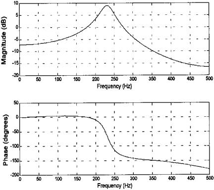
FIGURE 4.2 Plot of frequency characteristic (magnitude and phase) of the digital transfer function given above.

%of a linear digital system with the given digital

%transfer function

%Assume a sampling frequency of 1 kHz

Copyright 2004 by Marcel Dekker, Inc. All Rights Reserved.

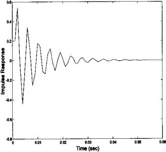
FIGURE 4.3 Impulse response of the digital transfer function described above. Both Figure 4.2 and Figure 4.3 were generated using the MATLAB code given in Example 1.

% Eq. (6)

Copyright 2004 by Marcel Dekker, Inc. All Rights Reserved.

xlabel(’Time (sec)’); ylabel (’Impulse Response’);

The digital filters described in the rest of this chapter use a straightforward application of these linear system concepts. The design and implementation of digital filters is merely a question of determining the a(n) and b(n) coefficients that produce linear processes with the desired frequency characteristics.

FINITE IMPULSE RESPONSE (FIR) FILTERS

FIR filters have transfer functions that have only numerator coefficients, i.e., H(z) = B(z). This leads to an impulse response that is finite, hence the name. They have the advantage of always being stable and having linear phase shifts. In addition, they have initial transients that are of finite durations and their extension to 2-dimensional applications is straightforward. The downside of FIR filters is that they are less efficient in terms of computer time and memory than IIR filters. FIR filters are also referred to as nonrecursive because only the input (not the output) is used in the filter algorithm (i.e., only the first term of Eq. (6) is used).

A simple FIR filter was developed in the context of Problem 3 in Chapter 2. This filter was achieved taking three consecutive points in the input array and averaging them together. The filter output was constructed by moving this threepoint average along the input waveform. For this reason, FIR filtering has also been referred to as a moving average process. (This term is used for any process that uses a moving set of multiplier weights, even if the operation does not really produce an average.) In Problem 4 of Chapter 2, this filter was implemented using a three weight filter, [1/3 1/3 1/3], which was convolved with the input waveform to produce the filtered output. These three numbers are simply the b(n) coefficients of a third-order, or three-weight, FIR filter. All FIR filters are similar to this filter; the only difference between them is the number and value of the coefficients.

The general equation for an FIR filter is a simplification of Eq. (6) and, after changing the limits to conform with MATLAB notation, becomes:

n=1

where b(n) is the coefficient function (also referred to as the weighting function) of length L, x(n) is the input, and y(n) is the output. This is identical to the convolution equation in Chapter 2 (Eq. (15)) with the impulse response, h(n),

Copyright 2004 by Marcel Dekker, Inc. All Rights Reserved.