Biosignal and Biomedical Image Processing MATLAB based Applications - John L. Semmlow

power spectrum of the filter’s output waveform. The parameters associated with the various approaches have been adjusted to produce as close a match to the filter transfer function as possible. The influence of some of these parameters is explored in the problems. The power spectrum produced by the classical approach is shown in Figure 5.7B and roughly approximates the spectral characteristics of the filter. The classical approach used the Welch method and averaged four segments with a maximum overlap. The model-based approach used the modified covariance method and a model order of 17, and produced a spectrum similar to that produced by the Welch method. The eigenvalue approach used a subspace of 13 and could only approximate the actual spectrum as a series of narrowband processes. This demonstrates that eigenvalue methods, while well-suited to identifying sinusoids in noise, are not good at estimating spectra that contain broader-band features.

PROBLEMS

1.Use sig_noise to generate a 254-point data segment containing two closely spaced sinusoids at 200 and 220 Hz both with SNR of -5 db. Find the best model order to distinguish these two peaks with a minimum of spurious peaks. Use the Burg method. Repeat with an SNR of -10 db.

2.Repeat Problem 1 above, but using a shorter data segment (N = 64), and a higher SNR: -1 db. Now lower the SNR to -5 db as in Problem 1 and note the severe degradation in performance.

3.Use sig_noise to generate a moderately long (N = 128) data segment consisting of a moderate (SNR = -5 db) sinusoid at 200 Hz and weak (SNR = -9 db) sinusoid at 230 Hz. Compare the spectrum generated by Welch, AR, and eigenvector methods.

4.Use the data in Problem 1 (SNR = −10db) to compare the operation of the pmusic and peig MATLAB algorithms. Use a signal space of 7 and 13 for each case. Plot power spectrum in db.

5.Use sig_noise to generate a short data segment (N = 64) containing two

closely spaced sinusoids in white noise (300 and 330 Hz). Both have SNR’s of −3 db. Compare the spectra obtained with the Welch, AR–Burg, and eigenvalue methods. For the AR model and eigenvector method chose a model or subspace order ranging between 5 to 19. Show the best case frequency plots.

6.Construct a broadband spectrum by passing white noise through a filter as in Example 5.4. Use the IIR bandpass filter of Example 4.7 (and Figure 4.16). Generate the filter’s transfer function directly from the coefficients, as in Exam-

Copyright 2004 by Marcel Dekker, Inc. All Rights Reserved.

ple 5.4. (Note you will have to take the FFT of both numerator and denominator coefficients and divide, or use freqz.) Next compare the spectrum produced by the three methods, as in Example 5.4. Adjust the parameters for the best relationship between the filter’s actual spectrum and that produced by the various methods.

Copyright 2004 by Marcel Dekker, Inc. All Rights Reserved.

6

Time–Frequency Analysis

BASIC APPROACHES

The spectral analysis techniques developed thus far represent powerful signal processing tools if one is not especially concerned with signal timing. Classical or modern spectral methods provide a complete and appropriate solution for waveforms that are stationary; that is, waveforms that do not change in their basic properties over the length of the analysis (strictly speaking, that do not change in their statistical properties). Yet many waveforms—particularly those of biological origin–are not stationary, and change substantially in their properties over time. For example, the EEG signal changes considerably depending on various internal states of the subject: i.e., meditation, sleep, eyes closed. Moreover, it is these changes with time that are often of primary interest. Fourier analysis provides a good description of the frequencies in a waveform, but not their timing. The Fourier transform “of a musical passage tells us what notes are played, but it is extremely different to figure out when they are played” (Hubbard, 1998). Such information must be embedded in the frequency spectrum since the Fourier transform is bilateral, and the musical passage can be uniquely reconstructed using the inverse Fourier transform. However, timing is encoded in the phase portion of the transform, and this encoding is difficult to interpret and recover. In the Fourier transform, specific events in time are distributed across all of the phase components. In essence, a local feature in time has been transformed into a global feature in phase.

Timing information is often of primary interest in many biomedical sig-

Copyright 2004 by Marcel Dekker, Inc. All Rights Reserved.

nals, and this is also true for medical images where the analogous information is localized in space. A wide range of approaches have been developed to try to extract both time and frequency information from a waveform. Basically they can be divided into two groups: time–frequency methods and time–scale methods. The latter are better known as Wavelet analyses, a popular new approach described in the next chapter. This chapter is dedicated to time–frequency methods.

Short-Term Fourier Transform: The Spectrogram

The first time–frequency methods were based on the straightforward approach of slicing the waveform of interest into a number of short segments and performing the analysis on each of these segments, usually using the standard Fourier transform. A window function similar to those described in Chapter 3 is applied to a segment of data, effectively isolating that segment from the overall waveform, and the Fourier transform is applied to that segment. This is termed the spectrogram or “short-term Fourier transform” (STFT)* since the Fourier Transform is applied to a segment of data that is shorter, often much shorter, than the overall waveform. Since abbreviated data segments are used, selecting the most appropriate window length can be critical. This method has been successfully applied in a number of biomedical applications.

The basic equation for the spectrogram in the continuous domain is:

where w(t-τ) is the window function and τ is the variable that slides the window across the waveform, x(t).

The discrete version of Eq. (1) is the same as was given in Chapter 2 for a general probing function (Eq. (11), Chapter 2) where the probing function is replaced by a family of sinusoids represented in complex format (i.e., e- jnm/N):

n=1

There are two main problems with the spectrogram: (1) selecting an optimal window length for data segments that contain several different features may not be possible, and (2) the time–frequency tradeoff: shortening the data length, N, to improve time resolution will reduce frequency resolution which is approximately 1/(NTs). Shortening the data segment could also result in the loss of low frequencies that are no longer fully included in the data segment. Hence, if the

*The terms STFT and spectrogram are used interchangeably and we will follow the same, slightly confusing convention here. Essentially the reader should be familiar with both terms.

Copyright 2004 by Marcel Dekker, Inc. All Rights Reserved.

window is made smaller to improve the time resolution, then the frequency resolution is degraded and visa versa. This time–frequency tradeoff has been equated to an uncertainty principle where the product of frequency resolution (expressed as bandwidth, B) and time, T, must be greater than some minimum. Specifically:

The trade-off between time and frequency resolution inherent in the STFT, or spectrogram, has motivated a number of other time–frequency methods as well as the time–scale approaches discussed in the next chapter. Despite these limitations, the STFT has been used successfully in a wide variety of problems, particularly those where only high frequency components are of interest and frequency resolution is not critical. The area of speech processing has benefitted considerably from the application of the STFT. Where appropriate, the STFT is a simple solution that rests on a well understood classical theory (i.e., the Fourier transform) and is easy to interpret. The strengths and weaknesses of the STFT are explored in the examples in the section on MATLAB Implementation below and in the problems at the end of the chapter.

Wigner-Ville Distribution: A Special Case of Cohen’s Class

A number of approaches have been developed to overcome some of the shortcomings of the spectrogram. The first of these was the Wigner-Ville distribution* which is also one of the most studied and best understood of the many time–frequency methods. The approach was actually developed by Wigner for use in physics, but later applied to signal processing by Ville, hence the dual name. We will see below that the Wigner-Ville distribution is a special case of a wide variety of similar transformations known under the heading of Cohen’s class of distributions. For an extensive summary of these distributions see Bou- dreaux-Bartels and Murry (1995).

The Wigner-Ville distribution, and others of Cohen’s class, use an approach that harkens back to the early use of the autocorrelation function for calculating the power spectrum. As noted in Chapter 3, the classic method for determining the power spectrum was to take the Fourier transform of the autocorrelation function (Eq. (14), Chapter 3). To construct the autocorrelation function, the waveform is compared with itself for all possible relative shifts, or lags (Eq. (16), Chapter 2). The equation is repeated here in both continuous and discreet form:

*The term distribution in this usage should more properly be density since that is the equivalent statistical term (Cohen, 1990).

Copyright 2004 by Marcel Dekker, Inc. All Rights Reserved.

k=1

where τ and n are the shift of the waveform with respect to itself.

In the standard autocorrelation function, time is integrated (or summed) out of the result, and this result, rxx(τ), is only a function of the lag, or shift, τ. The Wigner-Ville, and in fact all of Cohen’s class of distributions, use a variation of the autocorrelation function where time remains in the result. This is achieved by comparing the waveform with itself for all possible lags, but instead of integrating over time, the comparison is done for all possible values of time. This comparison gives rise to the defining equation of the so-called instantaneous autocorrelation function:

where τ and n are the time lags as in autocorrelation, and * represents the complex conjugate of the signal, x. Most actual signals are real, in which case Eq. (4) can be applied to either the (real) signal itself, or a complex version of the signal known as the analytic signal. A discussion of the advantages of using the analytic signal along with methods for calculating the analytic signal from the actual (i.e., real) signal is presented below.

The instantaneous autocorrelation function retains both lags and time, and is, accordingly, a two-dimensional function. The output of this function to a very simple sinusoidal input is shown in Figure 6.1 as both a three-dimensional and a contour plot. The standard autocorrelation function of a sinusoid would be a sinusoid of the same frequency. The instantaneous autocorrelation function output shown in Figure 6.1 shows a sinusoid along both the time and τ axis as expected, but also along the diagonals as well. These cross products are particularly apparent in Figure 6.1B and result from the multiplication in the instantaneous autocorrelation equation, Eq. (7). These cross products are a source of problems for all of the methods based on the instantaneous autocorrelation function.

As mentioned above, the classic method of computing the power spectrum was to take the Fourier transform of the standard autocorrelation function. The Wigner-Ville distribution echoes this approach by taking the Fourier transform

Copyright 2004 by Marcel Dekker, Inc. All Rights Reserved.

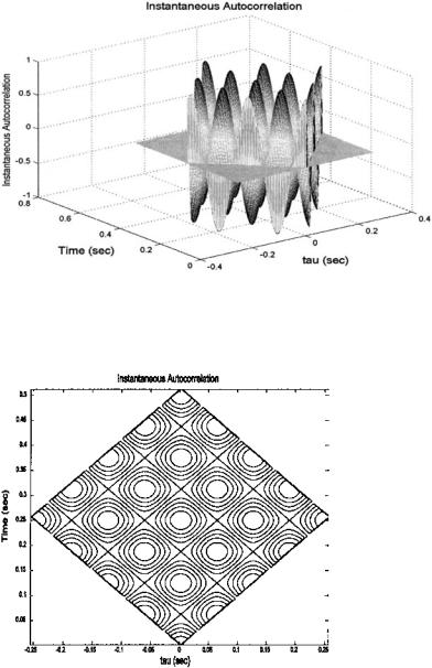
FIGURE 6.1A The instantaneous autocorrelation function of a two-cycle cosine wave plotted as a three-dimensional plot.

FIGURE 6.1B The instantaneous autocorrelation function of a two-cycle cosine wave plotted as a contour plot. The sinusoidal peaks are apparent along both axes as well as along the diagonals.

Copyright 2004 by Marcel Dekker, Inc. All Rights Reserved.

of the instantaneous autocorrelation function, but only along the τ (i.e., lag) dimension. The result is a function of both frequency and time. When the onedimensional power spectrum was computed using the autocorrelation function, it was common to filter the autocorrelation function before taking the Fourier transform to improve features of the resulting power spectrum. While no such filtering is done in constructing the Wigner-Ville distribution, all of the other approaches apply a filter (in this case a two-dimensional filter) to the instantaneous autocorrelation function before taking the Fourier transform. In fact, the primary difference between many of the distributions in Cohen’s class is simply the type of filter that is used.

The formal equation for determining a time–frequency distribution from Cohen’s class of distributions is rather formidable, but can be simplified in practice. Specifically, the general equation is:

where g(v,τ) provides the two-dimensional filtering of the instantaneous autocorrelation and is also know as a kernel. It is this filter-like function that differentiates between the various distributions in Cohen’s class. Note that the rest of the integrand is the Fourier transform of the instantaneous autocorrelation function.

There are several ways to simplify Eq. (8) for a specific kernel. For the Wigner-Ville distribution, there is no filtering, and the kernel is simply 1 (i.e., g(v,τ) = 1) and the general equation of Eq. (8), after integration by dv, reduces to Eq. (9), presented in both continuous and discrete form.

m=−∞

Note that t = nTs, and f = m/(NTs)

The Wigner-Ville has several advantages over the STFT, but also has a number of shortcomings. It greatest strength is that produces “a remarkably good picture of the time-frequency structure” (Cohen, 1992). It also has favorable marginals and conditional moments. The marginals relate the summation over time or frequency to the signal energy at that time or frequency. For example, if we sum the Wigner-Ville distribution over frequency at a fixed time, we get a value equal to the energy at that point in time. Alternatively, if we fix

Copyright 2004 by Marcel Dekker, Inc. All Rights Reserved.

frequency and sum over time, the value is equal to the energy at that frequency. The conditional moment of the Wigner-Ville distribution also has significance:

where p(t) is the marginal in time.

This conditional moment is equal to the so-called instantaneous frequency. The instantaneous frequency is usually interpreted as the average of the frequencies at a given point in time. In other words, treating the Wigner-Ville distribution as an actual probability density (it is not) and calculating the mean of frequency provides a term that is logically interpreted as the mean of the frequencies present at any given time.

The Wigner-Ville distribution has a number of other properties that may be of value in certain applications. It is possible to recover the original signal, except for a constant, from the distribution, and the transformation is invariant to shifts in time and frequency. For example, shifting the signal in time by a delay of T seconds would produce the same distribution except shifted by T on the time axis. The same could be said of a frequency shift (although biological processes that produce shifts in frequency are not as common as those that produce time shifts). These characteristics are also true of the STFT and some of the other distributions described below. A property of the Wigner-Ville distribution not shared by the STFT is finite support in time and frequency. Finite support in time means that the distribution is zero before the signal starts and after it ends, while finite support in frequency means the distribution does not contain frequencies beyond the range of the input signal. The Wigner-Ville does contain nonexistent energies due to the cross products as mentioned above and observed in Figure 6.1, but these are contained within the time and frequency boundaries of the original signal. Due to these cross products, the Wigner-Ville distribution is not necessarily zero whenever the signal is zero, a property Cohen called strong finite support. Obviously, since the STFT does not have finite support it does not have strong finite support. A few of the other distributions do have strong finite support. Examples of the desirable attributes of the Wigner-Ville will be explored in the MATLAB Implementation section, and in the problems.

The Wigner-Ville distribution has a number of shortcomings. Most serious of these is the production of cross products: the demonstration of energies at time–frequency values where they do not exist. These phantom energies have been the prime motivator for the development of other distributions that apply various filters to the instantaneous autocorrelation function to mitigate the damage done by the cross products. In addition, the Wigner-Ville distribution can have negative regions that have no meaning. The Wigner-Ville distribution also has poor noise properties. Essentially the noise is distributed across all time and

Copyright 2004 by Marcel Dekker, Inc. All Rights Reserved.

frequency including cross products of the noise, although in some cases, the cross products and noise influences can be reduced by using a window. In such cases, the desired window function is applied to the lag dimension of the instantaneous autocorrelation function (Eq. (7)) similar to the way it was applied to the time function in Chapter 3. As in Fourier transform analysis, windowing will reduce frequency resolution, and, in practice, a compromise is sought between a reduction of cross products and loss of frequency resolution. Noise properties and the other weaknesses of the Wigner-Ville distribution along with the influences of windowing are explored in the implementation and problem sections.

The Choi-Williams and Other Distributions

The existence of cross products in the Wigner-Ville transformation has motived the development of other distributions. These other distributions are also defined by Eq. (8); however, now the kernel, g(v,τ), is no longer 1. The general equation (Eq. (8)) can be simplified two different ways: for any given kernel, the integration with respect to the variable v can be performed in advance since the rest of the transform (i.e., the signal portion) is not a function of v; or use can be made of an intermediate function, called the ambiguity function.

In the first approach, the kernel is multiplied by the exponential in Eq. (9) to give a new function, G(u,τ):

where the new function, G(u,τ) is referred to as the determining function (Boashash and Reilly, 1992). Then Eq. (9) reduces to:

Note that the second set of terms under the double integral is just the instantaneous autocorrelation function given in Eq. (7). In terms of the determining function and the instantaneous autocorrelation function, the discrete form of Eq. (12) becomes:

τ=0

where t = u/fs. This is the approach that is used in the section on MATLAB implementation below. Alternatively, one can define a new function as the inverse Fourier transform of the instantaneous autocorrelation function:

Copyright 2004 by Marcel Dekker, Inc. All Rights Reserved.