Biosignal and Biomedical Image Processing MATLAB based Applications - John L. Semmlow

Figure 7.10 shows the waveform with a discontinuity in its second derivative at 0.5 sec. The lower trace indicates the position of the discontinuity. Note that the discontinuity is not visible in the waveform.

The output of the three-level analysis filter bank using the Daubechies 4- element filter is shown in Figure 7.11. The position of the discontinuity is clearly visible as a spike in the highpass subbands.

Feature Detection: Wavelet Packets

The DWT can also be used to construct useful descriptors of a waveform. Since the DWT is a bilateral transform, all of the information in the original waveform must be contained in the subband signals. These subband signals, or some aspect of the subband signals such as their energy over a given time period, could provide a succinct description of some important aspect of the original signal.

In the decompositions described above, only the lowpass filter subband signals were sent on for further decomposition, giving rise to the filter bank structure shown in the upper half of Figure 7.12. This decomposition structure is also known as a logarithmic tree. However, other decomposition structures are valid, including the complete or balanced tree structure shown in the lower half of Figure 7.12. In this decomposition scheme, both highpass and lowpass subbands are further decomposed into highpass and lowpass subbands up till the terminal signals. Other, more general, tree structures are possible where a decision on further decomposition (whether or not to split a subband signal) depends on the activity of a given subband. The scaling functions and wavelets associated with such general tree structures are known as wavelet packets.

Example 7.6 Apply balanced tree decomposition to the waveform consisting of a mixture of three equal amplitude sinusoids of 1 10 and 100 Hz. The main routine in this example is similar to that used in Examples 7.3 and 7.4 except that it calls the balanced tree decomposition routine, w_packet, and plots out the terminal waveforms. The w_packet routine is shown below and is used in this example to implement a 3-level decomposition, as illustrated in the lower half of Figure 7.12. This will lead to 8 output segments that are stored sequentially in the output vector, a.

%Example 7.5 and Figure 7.13

%Example of “Balanced Tree Decomposition”

%Construct a waveform of 4 sinusoids plus noise

%Decompose the waveform in 3 levels, plot outputs at the terminal

%level

Copyright 2004 by Marcel Dekker, Inc. All Rights Reserved.

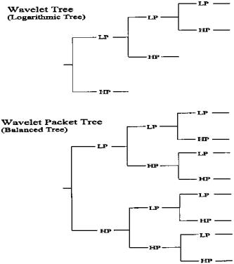
FIGURE 7.12 Structure of the analysis filter bank (wavelet tree) used in the DWT in which only the lowpass subbands are further decomposed and a more general structure in which all nonterminal signals are decomposed into highpass and lowpass subbands.

Copyright 2004 by Marcel Dekker, Inc. All Rights Reserved.

FIGURE 7.13 Balanced tree decomposition of the waveform shown in Figure 7.8. The signal from the upper left plot has been lowpass filtered 3 times and represents the lowest terminal signal in Figure 7.11. The upper right has been lowpass filtered twice then highpass filtered, and represents the second from the lowest terminal signal in Figure 7.11. The rest of the plots follow sequentially.

Copyright 2004 by Marcel Dekker, Inc. All Rights Reserved.

xlabel(’Time (sec)’);

end

The balanced tree decomposition routine, w_packet, operates similarly to the DWT analysis filter banks, except for the filter structure. At each level, signals from the previous level are isolated, filtered (using standard convolution), downsampled, and both the highand lowpass signals overwrite the single signal from the previous level. At the first level, the input waveform is replaced by the filtered, downsampled highand lowpass signals. At the second level, the two highand lowpass signals are each replaced by filtered, downsampled highand lowpass signals. After the second level there are now four sequential signals in the original data array, and after the third level there be will be eight.

%Function to generate a “balanced tree” filter bank

%All arguments are the same as in routine ‘analyze’

%an = w_packet(x,h,L)

%where

% x = input waveform (must be longer than 2vL L and power of

%two)

%h0 = filter coefficients (low pass)

%L = decomposition level (number of High pass filter in bank)

function an = w_packet(x,h0,L)

% Calculate High pass coefficients from low pass coefficients

Copyright 2004 by Marcel Dekker, Inc. All Rights Reserved.

The output produced by this decomposition is shown in Figure 7.13. The filter bank outputs emphasize various components of the three-sine mixture. Another example is given in Problem 7 using a chirp signal.

One of the most popular applications of the dyadic wavelet transform is in data compression, particularly of images. However, since this application is not so often used in biomedical engineering (although there are some applications regrading the transmission of radiographic images), it will not be covered here.

PROBLEMS

1.(A) Plot the frequency characteristics (magnitude and phase) of the Mexican hat and Morlet wavelets.

(B) The plot of the phase characteristics will be incorrect due to phase wrapping.

Phase wrapping is due to the fact that the arctan function can never be greater that ± 2π; hence, once the phase shift exceeds ± 2π (usually minus), it warps around and appears as positive. Replot the phase after correcting for this wrap-

around effect. (Hint: Check for discontinuities above a certain amount, and when that amount is exceeded, subtract 2π from the rest of the data array. This is a simple algorithm that is generally satisfactory in linear systems analysis.)

2.Apply the continuous wavelet analysis used in Example 7.1 to analyze a chirp signal running between 2 and 30 Hz over a 2 sec period. Assume a sample rate of 500 Hz as in Example 7.1. Use the Mexican hat wavelet. Show both contour and 3-D plot.

3.Plot the frequency characteristics (magnitude and phase) of the Haar and Daubechies 4-and 10-element filters. Assume a sample frequency of 100 Hz.

Copyright 2004 by Marcel Dekker, Inc. All Rights Reserved.

4.Generate a Daubechies 10-element filter and plot the magnitude spectrum as in Problem 3. Construct the highpass filter using the alternating flip algorithm (Eq. (20)) and plot its magnitude spectrum. Generate the lowpass and highpass synthesis filter coefficients using the order flip algorithm (Eqs. (23) and (24)) and plot their respective frequency characteristics. Assume a sampling frequency of 100 Hz.

5.Construct a waveform of a chirp signal as in Problem 2 plus noise. Make the variance of the noise equal to the variance of the chirp. Decompose the waveform in 5 levels, operate on the lowest level (i.e., the high resolution highpass signal), then reconstruct. The operation should zero all elements below a given threshold. Find the best threshold. Plot the signal before and after reconstruction. Use Daubechies 6-element filter.

6.Discontinuity detection. Load the waveform x in file Prob7_6_data which consists of a waveform of 2 sinusoids the same as in Figure 7.9, but with a series of diminishing discontinuities in the second derivative. The discontinuities in the second derivative begin at approximately 0.5% of the sinusoidal amplitude and decrease by a factor of 2 for each pair of discontinuities. (The offset array can be obtained in the variable offset.) Decompose the waveform into three levels and examine and plot only the highest resolution highpass filter output to detect the discontinuity. Hint: The highest resolution output will be located in N/2 to N of the analysis output array. Use a Harr and a Daubechies 10-element filter and compare the difference in detectability. (Note that the Haar is a very weak filter so that some of the low frequency components will still be found in its output.)

7.Apply the balanced tree decomposition to a chirp signal similar to that used in Problem 5 except that the chirp frequency should range between 2 and 100 Hz. Decompose the waveform into 3 levels and plot the outputs at the terminal level as in Example 7.5. Use a Daubechies 4-element filter. Note that each output filter responds to different portions of the chirp signal.

Copyright 2004 by Marcel Dekker, Inc. All Rights Reserved.

8

Advanced Signal Processing

Techniques: Optimal

and Adaptive Filters

OPTIMAL SIGNAL PROCESSING: WIENER FILTERS

The FIR and IIR filters described in Chapter 4 provide considerable flexibility in altering the frequency content of a signal. Coupled with MATLAB filter design tools, these filters can provide almost any desired frequency characteristic to nearly any degree of accuracy. The actual frequency characteristics attained by the various design routines can be verified through Fourier transform analysis. However, these design routines do not tell the user what frequency characteristics are best; i.e., what type of filtering will most effectively separate out signal from noise. That decision is often made based on the user’s knowledge of signal or source properties, or by trial and error. Optimal filter theory was developed to provide structure to the process of selecting the most appropriate frequency characteristics.

A wide range of different approaches can be used to develop an optimal filter, depending on the nature of the problem: specifically, what, and how much, is known about signal and noise features. If a representation of the desired signal is available, then a well-developed and popular class of filters known as Wiener filters can be applied. The basic concept behind Wiener filter theory is to minimize the difference between the filtered output and some desired output. This minimization is based on the least mean square approach, which adjusts the filter coefficients to reduce the square of the difference between the desired and actual waveform after filtering. This approach requires

Copyright 2004 by Marcel Dekker, Inc. All Rights Reserved.

FIGURE 8.1 Basic arrangement of signals and processes in a Wiener filter.

an estimate of the desired signal which must somehow be constructed, and this estimation is usually the most challenging aspect of the problem.*

The Wiener filter approach is outlined in Figure 8.1. The input waveform containing both signal and noise is operated on by a linear process, H(z). In practice, the process could be either an FIR or IIR filter; however, FIR filters are more popular as they are inherently stable,† and our discussion will be limited to the use of FIR filters. FIR filters have only numerator terms in the transfer function (i.e., only zeros) and can be implemented using convolution first presented in Chapter 2 (Eq. (15)), and later used with FIR filters in Chapter 4 (Eq. (8)). Again, the convolution equation is:

k=1

where h(k) is the impulse response of the linear filter. The output of the filter, y(n), can be thought of as an estimate of the desired signal, d(n). The difference between the estimate and desired signal, e(n), can be determined by simple subtraction: e(n) = d(n) − y(n).

As mentioned above, the least mean square algorithm is used to minimize the error signal: e(n) = d(n) − y(n). Note that y(n) is the output of the linear filter, H(z). Since we are limiting our analysis to FIR filters, h(k) ≡ b(k), and e(n) can be written as:

k=0

where L is the length of the FIR filter. In fact, it is the sum of e(n)2 which is minimized, specifically:

*As shown below, only the crosscorrelation between the unfiltered and the desired output is necessary for the application of these filters.

†IIR filters contain internal feedback paths and can oscillate with certain parameter combinations.

Copyright 2004 by Marcel Dekker, Inc. All Rights Reserved.

After squaring the term in brackets, the sum of error squared becomes a quadratic function of the FIR filter coefficients, b(k), in which two of the terms can be identified as the autocorrelation and cross correlation:

where, from the original definition of crossand autocorrelation (Eq. (3), Chap- ter 2):

L

rdx(k) = ∑ d(R) x(R + k)

R=1

L

rxx(k) = ∑ x(R) x(R + k)

R=1

Since we desire to minimize the error function with respect to the FIR filter coefficients, we take derivatives with respect to b(k) and set them to zero:

k=1

Equation (5) shows that the optimal filter can be derived knowing only the autocorrelation function of the input and the crosscorrelation function between the input and desired waveform. In principle, the actual functions are not necessary, only the autoand crosscorrelations; however, in most practical situations the autoand crosscorrelations are derived from the actual signals, in which case some representation of the desired signal is required.

To solve for the FIR coefficients in Eq. (5), we note that this equation actually represents a series of L equations that must be solved simultaneously. The matrix expression for these simultaneous equations is:

Equation (6) is commonly known as the Wiener-Hopf equation and is a basic component of Wiener filter theory. Note that the matrix in the equation is

Copyright 2004 by Marcel Dekker, Inc. All Rights Reserved.

FIGURE 8.2 Configuration for using optimal filter theory for systems identification.

the correlation matrix mentioned in Chapter 2 (Eq. (21)) and has a symmetrical structure termed a Toeplitz structure.* The equation can be written more succinctly using standard matrix notation, and the FIR coefficients can be obtained by solving the equation through matrix inversion:

The application and solution of this equation are given for two different examples in the following section on MATLAB implementation.

The Wiener-Hopf approach has a number of other applications in addition to standard filtering including systems identification, interference canceling, and inverse modeling or deconvolution. For system identification, the filter is placed in parallel with the unknown system as shown in Figure 8.2. In this application, the desired output is the output of the unknown system, and the filter coefficients are adjusted so that the filter’s output best matches that of the unknown system. An example of this application is given in a subsequent section on adaptive signal processing where the least mean squared (LMS) algorithm is used to implement the optimal filter. Problem 2 also demonstrates this approach. In interference canceling, the desired signal contains both signal and noise while the filter input is a reference signal that contains only noise or a signal correlated with the noise. This application is also explored under the section on adaptive signal processing since it is more commonly implemented in this context.

MATLAB Implementation

The Wiener-Hopf equation (Eqs. (5) and (6), can be solved using MATLAB’s matrix inversion operator (‘\’) as shown in the examples below. Alternatively,

*Due to this matrix’s symmetry, it can be uniquely defined by only a single row or column.

Copyright 2004 by Marcel Dekker, Inc. All Rights Reserved.