

Biosignal and Biomedical Image Processing MATLAB based Applications - John L. Semmlow
.pdfFIGURE 7.8 Signals generated by the analysis filter bank used in Example 7.3 with the top-most plot showing the outputs of the first set of filters with the finest resolution, the next from the top showing the outputs of the second set of set of filters, etc. Only the lowest (i.e., smoothest) lowpass subband signal is included in the output of the filter bank; the rest are used only in the determination of highpass subbands. The lowest plots show the frequency characteristics of the highand lowpass filters.
% |
|
|
|
[x t] = signal(freqsin,ampl,N); |
% Construct signal |
||
x1 = |
x (.25 * randn(1,N)); |
% Add noise |
|
an = |
analyze(x1,h0,4); |
% Decompose signal, |
|
|
|
% |
analytic filter bank |
sy = |
synthesize(an,h0,4); |
% Reconstruct original |
|
|
|
% |
signal |
figure(fig1);
plot(t,x,’k’,t,x1–4,’k’,t,sy-8,’k’);% Plot signals separated
Copyright 2004 by Marcel Dekker, Inc. All Rights Reserved.
This program uses the function signal to generate the mixtures of sinusoids. This routine is similar to sig_noise except that it generates only mixtures of sine waves without the noise. The first argument specifies the frequency of the sines and the third argument specifies the number of points in the waveform just as in sig_noise. The second argument specifies the amplitudes of the sinusoids, not the SNR as in sig_noise.
The analysis function shown below implements the analysis filter bank. This routine first generates the highpass filter coefficients, h1, from the lowpass filter coefficients, h, using the alternating flip algorithm of Eq. (20). These FIR filters are then applied using standard convolution. All of the various subband signals required for reconstruction are placed in a single output array, an. The length of an is the same as the length of the input, N = 1024 in this example. The only lowpass signal needed for reconstruction is the smoothest lowpass subband (i.e., final lowpass signal in the lowpass chain), and this signal is placed in the first data segment of an taking up the first N/16 data points. This signal is followed by the last stage highpass subband which is of equal length. The next N/8 data points contain the second to last highpass subband followed, in turn, by the other subband signals up to the final, highest resolution highpass subband which takes up all of the second half of an. The remainder of the analyze routine calculates and plots the highand lowpass filter frequency characteristics.
%Function to calculate analyze filter bank
%an = analyze(x,h,L)
%where
%x = input waveform in column form which must be longer than
%2vL L and power of two.
%h0 = filter coefficients (lowpass)
%L = decomposition level (number of highpass filter in bank)
function an = analyze(x,h0,L)
lf = |
length(h0); |
% Filter length |
|
lx |
= |
length(x); |
% Data length |
an |
= |
x; |
% Initialize output |
%Calculate High pass coefficients from low pass coefficients for i = 0:(lf-1)
h1(i 1) = (-1)vi * h0(lf-i); % Alternating flip, Eq. (20) end
%Calculate filter outputs for all levels
for i = 1:L a_ext = an;
Copyright 2004 by Marcel Dekker, Inc. All Rights Reserved.
lpf = conv(a_ext,h0); |
% Lowpass FIR filter |
|
hpf = conv(a_ext,h1); |
% Highpass FIR filter |
|
lpf = |
lpf(1:lx); |
% Remove extra points |
hpf = |
hpf(1:lx); |
|
lpfd = |
lpf(1:2:end); |
% Downsample |
hpfd = |
hpf(1:2:end); |
|
an(1:lx) = [lpfd hpfd]; |
% Low pass output at beginning |
|
|
|
% of array, but now occupies |
|
|
% only half the data |
|
|
% points as last pass |
lx = lx/2; |
|
|
subplot(L 1,2,2*i-1); |
% Plot both filter outputs |
|
plot(an(1:lx)); |
% Lowpass output |
|
if i == 1
title(’Low Pass Outputs’); % Titles end
subplot(L 1,2,2*i);
plot(an(lx 1:2*lx)); if i == 1
title(’High Pass Outputs’)
end end
%
HPF = abs(fft(h1,256)); LPF = abs(fft(h0,256));
freq = (1:128)* 1000/256; subplot(L 1,2,2*i 1);
plot(freq, LPF(1:128)); % Plot from 0 to fs/2 Hz text(1,1.7,’Low Pass Filter’);
xlabel(’Frequency (Hz.)’)’ subplot(L 1,2,2*i 2);
plot(freq, HPF(1:128));
text(1,1.7,’High Pass Filter’);
xlabel(’Frequency (Hz.)’)’
The original data are reconstructed from the analyze filter bank signals in the program synthesize. This program first constructs the synthesis lowpass filter, g0, using order flip applied to the analysis lowpass filter coefficients (Eq. (23)). The analysis highpass filter is constructed using the alternating flip algorithm (Eq. (20)). These coefficients are then used to construct the synthesis highpass filter coefficients through order flip (Eq. (24)). The synthesis filter loop begins with the course signals first, those in the initial data segments of a with the shortest segment lengths. The lowpass and highpass signals are upsampled, then filtered using convolution, the additional points removed, and the signals added together. This loop is structured so that on the next pass the
Copyright 2004 by Marcel Dekker, Inc. All Rights Reserved.
recently combined segment is itself combined with the next higher resolution highpass signal. This iterative process continues until all of the highpass signals are included in the sum.
%Function to calculate synthesize filter bank
%y = synthesize(a,h0,L)
%where
%a = analyze filter bank outputs (produced by analyze)
%h = filter coefficients (lowpass)
%L = decomposition level (number of highpass filters in bank)
function y = synthesize(a,h0,L)
lf = |
length(h0); |
% Filter length |
lx = |
length(a); |
% Data length |
lseg = lx/(2vL); |
% Length of first lowand |
|
|
|
% highpass segments |
y = |
a; |
% Initialize output |
g0 = |
h0(lf:-1:1); |
% Lowpass coefficients using |
% order flip, Eq. (23)
%Calculate High pass coefficients, h1(n), from lowpass
%coefficients use Alternating flip Eq. (20) for i = 0:(lf-1)
h1(i 1) = (-1)vi * h0(lf-i); |
|
|
|
end |
|
|
|
g1 = h1(lf:-1:1); |
% Highpass filter coeffi- |
||
|
|
% |
cients using order |
|
|
% |
flip, Eq. (24) |
% Calculate filter outputs for all levels |
|||
for i = |
1:L |
|
|
lpx = |
y(1:lseg); |
% Get lowpass segment |
|
hpx = y(lseg 1:2*lseg); |
% Get highpass outputs |
||
up_lpx = zeros(1,2*lseg); |
% Initialize for upsampling |
||
up_lpx(1:2:2*lseg) = lpx; |
% Upsample lowpass (every |
||
|
|
% |
odd point) |
up_hpx = zeros(1,2*lseg); |
% Repeat for highpass |
||
up_hpx(1:2:2*lseg) = hpx; |
|
|
|
syn = |
conv(up_lpx,g0) conv(up_hpx,g1); % Filter and |
||
|
|
|
% combine |
y(1:2*lseg) = syn(1:(2*lseg)); % Remove extra points from |
|||
|
|
% |
end |
lseg = lseg * 2; |
% Double segment lengths for |
||
|
|
% |
next pass |
end |
|
|
|
The subband signals are shown in Figure 7.8. Also shown are the frequency characteristics of the Daubechies highand lowpass filters. The input
Copyright 2004 by Marcel Dekker, Inc. All Rights Reserved.
and reconstructed output waveforms are shown in Figure 7.7. The original signal before the noise was added is included. Note that the reconstructed waveform closely matches the input except for the phase lag introduced by the filters. As shown in the next example, this phase lag can be eliminated by using circular or periodic convolution, but this will also introduce some artifact.
Denoising
Example 7.3 was not particularly practical since the reconstructed signal was the same as the original, except for the phase shift. A more useful application of wavelets is shown in Example 7.4, where some processing is done on the subband signals before reconstruction—in this example, nonlinear filtering. The basic assumption in this application is that the noise is coded into small fluctuations in the higher resolution (i.e., more detailed) highpass subbands. This noise can be selectively reduced by eliminating the smaller sample values in the higher resolution highpass subbands. In this example, the two highest resolution highpass subbands are examined and data points below some threshold are zeroed out. The threshold is set to be equal to the variance of the highpass subbands.
Example 7.4 Decompose the signal in Example 7.3 using a 4-level filter bank. In this example, use periodic convolution in the analysis and synthesis filters and a 4-element Daubechies filter. Examine the two highest resolution highpass subbands. These subbands will reside in the last N/4 to N samples. Set all values in these segments that are below a given threshold value to zero. Use the net variance of the subbands as the threshold.
%Example 7.4 and Figure 7.9
%Application of DWT to nonlinear filtering
%Construct the waveform in Example 7.3.
%Decompose the waveform in 4 levels, plot each level, then
%reconstruct.
%Use Daubechies 4-element filter and periodic convolution.
%Evaluate the two highest resolution highpass subbands and
%zero out those samples below some threshold value.
%
close all; clear all; fs = 1000;
N = 1024;
%
freqsin = [.63 1.1 2.7 5.6]; ampl = [1.2 1 1.2 .75 ];
[x t] = signal(freqsin,ampl,N); x = x (.25 * randn(1,N));
h0 = daub(4); figure(fig1);
Copyright 2004 by Marcel Dekker, Inc. All Rights Reserved.
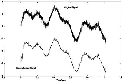
FIGURE 7.9 Application of the dyadic wavelet transform to nonlinear filtering. After subband decomposition using an analysis filter bank, a threshold process is applied to the two highest resolution highpass subbands before reconstruction using a synthesis filter bank. Periodic convolution was used so that there is no phase shift between the input and output signals.
an = analyze1(x,h0,4); |
% Decompose signal, analytic |
|
% filter bank of level 4 |
%Set the threshold times to equal the variance of the two higher
%resolution highpass subbands.
threshold = var(an(N/4:N)); for i = (N/4:N)
if an(i) < threshold an(i) = 0;
end end
sy = synthesize1(an,h0,4);
figure(fig2); plot(t,x,’k’,t,sy-5,’k’);
axis([-.2 1.2-8 4]); xlabel(’Time(sec)’)
Copyright 2004 by Marcel Dekker, Inc. All Rights Reserved.
The routines for the analysis and synthesis filter banks differ slightly from those used in Example 7.3 in that they use circular convolution. In the analysis filter bank routine (analysis1), the data are first extended using the periodic or wraparound approach: the initial points are added to the end of the original data sequence (see Figure 2.10B). This extension is the same length as the filter. After convolution, these added points and the extra points generated by convolution are removed in a symmetrical fashion: a number of points equal to the filter length are removed from the initial portion of the output and the remaining extra points are taken off the end. Only the code that is different from that shown in Example 7.3 is shown below. In this code, symmetric elimination of the additional points and downsampling are done in the same instruction.
function an = analyze1(x,h0,L)..........
........... |
|
|
for i = 1:L |
|
|
a_ext = [an an(1:lf)]; |
% Extend data for “periodic |
|
|
% |
convolution” |
lpf = conv(a_ext,h0); |
% Lowpass FIR filter |
|
hpf = conv(a_ext,h1); |
% Highpass FIR filter |
|
lpfd = lpf(lf:2:lf lx-1); |
% Remove extra points. Shift to |
|
hpfd = hpf(lf:2:lf lx-1); |
% obtain circular segment; then |
|
|
% |
downsample |
an(1:lx) = [lpfd hpfd]; |
% Lowpass output at beginning of |
|
|
% array, but now occupies only |
|
|
% half the data points as last |
|
|
% |
pass |
lx = lx/2; .....................
The synthesis filter bank routine is modified in a similar fashion except that the initial portion of the data is extended, also in wraparound fashion (by adding the end points to the beginning). The extended segments are then upsampled, convolved with the filters, and added together. The extra points are then removed in the same manner used in the analysis routine. Again, only the modified code is shown below.
function y = synthesize1(an,h0,L) |
...................... |
|
............. |
|
|
for i = |
1:L |
|
lpx = |
y(1:lseg); |
% Get lowpass segment |
hpx = |
y(lseg 1:2*lseg); |
% Get highpass outputs |
lpx = |
[lpx(lseg-lf/2 1:lseg) lpx]; % Circular extension: |
|
|
|
% lowpass comp. |
hpx = |
[hpx(lseg-lf/2 1:lseg) hpx]; % and highpass component |
|
l_ext = length(lpx);
Copyright 2004 by Marcel Dekker, Inc. All Rights Reserved.
up_lpx = zeros(1,2*l_ext); |
% Initialize vector for |
||
|
% |
upsampling |
|
up_lpx(1:2:2*l_ext) = lpx; |
% Up sample lowpass (every |
||
|
% |
odd point) |
|
up_hpx = zeros(1,2*l_ext); |
% Repeat for highpass |
||
up_hpx(1:2:2*l_ext) = hpx; |
|
|
|
syn = conv(up_lpx,g0) conv(up_hpx,g1); |
% Filter and |
||
|
|
|
% combine |
y(1:2*lseg) = syn(lf 1:(2*lseg) lf); % Remove extra |
|||
|
|
% |
points |
lseg = lseg * 2; |
% Double segment lengths |
||
|
% |
for next pass |
|
end
.........................
The original and reconstructed waveforms are shown in Figure 7.9. The filtering produced by thresholding the highpass subbands is evident. Also there is no phase shift between the original and reconstructed signal due to the use of periodic convolution, although a small artifact is seen at the beginning and end of the data set. This is because the data set was not really periodic.
Discontinuity Detection
Wavelet analysis based on filter bank decomposition is particularly useful for detecting small discontinuities in a waveform. This feature is also useful in image processing. Example 7.5 shows the sensitivity of this method for detecting small changes, even when they are in the higher derivatives.
Example 7.5 Construct a waveform consisting of 2 sinusoids, then add a small (approximately 1% of the amplitude) offset to this waveform. Create a new waveform by double integrating the waveform so that the offset is in the second derivative of this new signal. Apply a three-level analysis filter bank. Examine the high frequency subband for evidence of the discontinuity.
%Example 7.5 and Figures 7.10 and 7.11. Discontinuity detection
%Construct a waveform of 2 sinusoids with a discontinuity
%in the second derivative
%Decompose the waveform into 3 levels to detect the
%discontinuity.
%Use Daubechies 4-element filter
% |
|
|
close all; clear all; |
|
|
fig1 = |
figure(’Units’,’inches’,’Position’,[0 2.5 3 3.5]); |
|
fig2 = |
figure(’Units’, ’inches’,’Position’,[3 2.5 5 5]); |
|
fs = 1000; |
% Sample frequency |
|
Copyright 2004 by Marcel Dekker, Inc. All Rights Reserved.
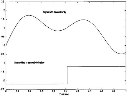
FIGURE 7.10 Waveform composed of two sine waves with an offset discontinuity in its second derivative at 0.5 sec. Note that the discontinuity is not apparent in the waveform.
N = |
1024; |
% Number of points in |
||
|
|
|
% |
waveform |
freqsin = [.23 .8 1.8]; |
% Sinusoidal frequencies |
|||
ampl = |
[1.2 1 .7]; |
% Amplitude of sinusoid |
||
incr = |
.01; |
% Size of second derivative |
||
|
|
|
% |
discontinuity |
offset = [zeros(1,N/2) ones(1,N/2)]; |
||||
h0 = |
daub(4) |
% Daubechies 4 |
||
% |
|
|
|
|
[x1 t] = signal(freqsin,ampl,N); |
% Construct signal |
|||
x1 = |
x1 offset*incr; |
% Add discontinuity at |
||
|
|
|
% |
midpoint |
x = |
integrate(integrate(x1)); |
% Double integrate |
||
figure(fig1);
plot(t,x,’k’,t,offset-2.2,’k’); % Plot new signal axis([0 1-2.5 2.5]);
xlabel(’Time (sec)’);
Copyright 2004 by Marcel Dekker, Inc. All Rights Reserved.
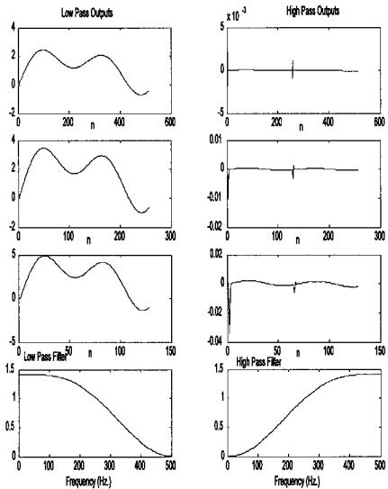
FIGURE 7.11 Analysis filter bank output of the signal shown in Figure 7.10. Although the discontinuity is not visible in the original signal, its presence and location are clearly identified as a spike in the highpass subbands.
Copyright 2004 by Marcel Dekker, Inc. All Rights Reserved.