

Biosignal and Biomedical Image Processing MATLAB based Applications - John L. Semmlow
.pdfFIGURE 8.7 Configuration for adaptive noise cancellation. The reference channel carries a signal, N’(n), that is correlated with the noise, N(n), but not with the signal of interest, x(n). The adaptive filter produces an estimate of the noise, N*(n), that is in the signal. In some applications, multiple reference channels are used to provide a more accurate representation of the background noise.
MATLAB Implementation
The implementation of the LMS recursive algorithm (Eq. (11)) in MATLAB is straightforward and is given below. Its application is illustrated through several examples below.
The LMS algorithm is implemented in the function
function [b,y,e] = |
lms(x,d,delta,L) |
|
% |
|
|
% Inputs: |
x = |
input |
% |
d = |
desired signal |
% |
delta = the convergence gain |
|
% |
L is the length (order) of the FIR filter |
|
% Outputs: |
b = |
FIR filter coefficients |
% |
y = |
ALE output |
% |
e = |
residual error |
%Simple function to adjust filter coefficients using the LSM
%algorithm
%Adjusts filter coefficients, b, to provide the best match
%between the input, x(n), and a desired waveform, d(n),
%Both waveforms must be the same length
%Uses a standard FIR filter
% |
|
|
M |
= |
length(x); |
b |
= |
zeros(1,L); y = zeros(1,M); % Initialize outputs |
for n = L:M
Copyright 2004 by Marcel Dekker, Inc. All Rights Reserved.
x1 = x(n:-1:n-L 1); |
% Select input for convolu- |
||
|
|
% |
tion |
y(n) = |
b * x1’; |
% Convolve (multiply) |
|
|
|
% |
weights with input |
e(n) = |
d(n)—y(n); |
% Calculate error |
|
b = b delta*e(n)*x1; |
% Adjust weights |
||
end
Note that this function operates on the data as block, but could easily be modified to operate on-line, that is, as the data are being acquired. The routine begins by applying the filter with the current coefficients to the first L points (L is the filter length), calculates the error between the filter output and the desired output, then adjusts the filter coefficients accordingly. This process is repeated for another data segment L-points long, beginning with the second point, and continues through the input waveform.
Example 8.3 Optimal filtering using the LMS algorithm. Given the same sinusoidal signal in noise as used in Example 8.1, design an adaptive filter to remove the noise. Just as in Example 8.1, assume that you have a copy of the desired signal.
Solution The program below sets up the problem as in Example 8.1, but uses the LMS algorithm in the routine lms instead of the Wiener-Hopf equation.
%Example 8.3 and Figure 8.8 Adaptive Filters
%Use an adaptive filter to eliminate broadband noise from a
%narrowband signal
%Use LSM algorithm applied to the same data as Example 8.1
close all; clear all;
fs = |
1000;*IH26* |
% Sampling frequency |
N = |
1024; |
% Number of points |
L = |
256; |
% Optimal filter order |
a = |
.25; |
% Convergence gain |
% |
|
|
% Same initial lines as in Example 8.1 ..... |
||
%% Calculate convergence parameter |
||
PX = |
(1/(N 1))* sum(xn.v2); % Calculate approx. power in xn |
|
delta = a * (1/(10*L*PX)); |
% Calculate |
|
b = |
lms(xn,x,delta,L); |
% Apply LMS algorithm (see below) |
%
% Plotting identical to Example 8.1. ...
Example 8.3 produces the data in Figure 8.8. As with the Wiener filter, the adaptive process adjusts the FIR filter coefficients to produce a narrowband filter centered about the sinusoidal frequency. The convergence factor, a, was
Copyright 2004 by Marcel Dekker, Inc. All Rights Reserved.
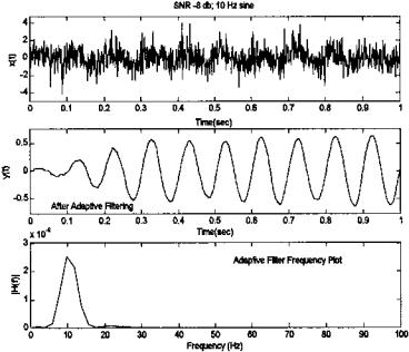
FIGURE 8.8 Application of an adaptive filter using the LSM recursive algorithm to data containing a single sinusoid (10 Hz) in noise (SNR = -8 db). Note that the filter requires the first 0.4 to 0.5 sec to adapt (400–500 points), and that the frequency characteristics of the coefficients produced after adaptation are those of a bandpass filter with a single peak at 10 Hz. Comparing this figure with Figure 8.3 suggests that the adaptive approach is somewhat more effective than the Wiener filter for the same number of filter weights.
empirically set to give rapid, yet stable convergence. (In fact, close inspection of Figure 8.8 shows a small oscillation in the output amplitude suggesting marginal stability.)
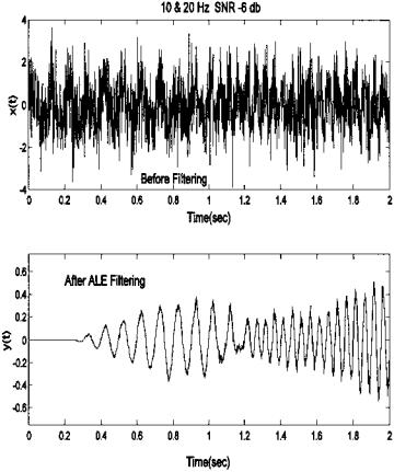
Example 8.4 The application of the LMS algorithm to a stationary signal was given in Example 8.3. Example 8.4 explores the adaptive characteristics of algorithm in the context of an adaptive line enhancement problem. Specifically, a single sinusoid that is buried in noise (SNR = -6 db) abruptly changes frequency. The ALE-type filter must readjust its coefficients to adapt to the new frequency.
The signal consists of two sequential sinusoids of 10 and 20 Hz, each lasting 0.6 sec. An FIR filter with 256 coefficients will be used. Delay and convergence gain will be set for best results. (As in many problems some adjustments must be made on a trial and error basis.)
Copyright 2004 by Marcel Dekker, Inc. All Rights Reserved.
Solution Use the LSM recursive algorithm to implement the ALE filter.
%Example 8.4 and Figure 8.9 Adaptive Line Enhancement (ALE)
%Uses adaptive filter to eliminate broadband noise from a
%narrowband signal
% |
|
% Generate signal and noise |
|
close all; clear all; |
|
fs = 1000; |
% Sampling frequency |
FIGURE 8.9 Adaptive line enhancer applied to a signal consisting of two sequential sinusoids having different frequencies (10 and 20 Hz). The delay of 5 samples and the convergence gain of 0.075 were determined by trial and error to give the best results with the specified FIR filter length.
Copyright 2004 by Marcel Dekker, Inc. All Rights Reserved.
L = |
256; |
% Filter order |
|
N = |
2000; |
% Number of points |
|
delay = 5; |
% Decorrelation delay |
||
a |
= |
.075; |
% Convergence gain |
t |
= |
(1:N)/fs; |
% Time vector for plotting |
%
%Generate data: two sequential sinusoids, 10 & 20 Hz in noise
%(SNR = -6)
x = [sig_noise(10,-6,N/2) sig_noise(20,-6,N/2)];
% |
|
|
subplot(2,1,1); |
% Plot unfiltered data |
|
plot(t, x,’k’); |
|
|
........axis, title............. |
|
|
PX = (1/(N 1))* sum(x.v2); |
% Calculate waveform |
|
|
% |
power for delta |
delta = (1/(10*L*PX)) * a; |
% Use 10% of the max. |
|
|
% |
range of delta |
xd = [x(delay:N) zeros(1,delay-1)]; |
% Delay signal to decor- |
|
|
% |
relate broadband noise |
[b,y] = lms(xd,x,delta,L); |
% Apply LMS algorithm |
|
subplot(2,1,2); |
% Plot filtered data |
|
plot(t,y,’k’); |
|
|
........axis, title.............. |
|
|
The results of this code are shown in Figure 8.9. Several values of delay were evaluated and the delay chosen, 5 samples, showed marginally better results than other delays. The convergence gain of 0.075 (7.5% maximum) was also determined empirically. The influence of delay on ALE performance is explored in Problem 4 at the end of this chapter.
Example 8.5 The application of the LMS algorithm to adaptive noise cancellation is given in this example. Here a single sinusoid is considered as noise and the approach reduces the noise produced the sinusoidal interference signal. We assume that we have a scaled, but otherwise identical, copy of the interference signal. In practice, the reference signal would be correlated with, but not necessarily identical to, the interference signal. An example of this more practical situation is given in Problem 5.
%Example 8.5 and Figure 8.10 Adaptive Noise Cancellation
%Use an adaptive filter to eliminate sinusoidal noise from a
%narrowband signal
%
% Generate signal and noise close all; clear all;
Copyright 2004 by Marcel Dekker, Inc. All Rights Reserved.
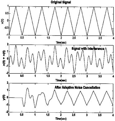
FIGURE 8.10 Example of adaptive noise cancellation. In this example the reference signal was simply a scaled copy of the sinusoidal interference, while in a more practical situation the reference signal would be correlated with, but not identical to, the interference. Note the near perfect cancellation of the interference.
fs = |
500; |
% Sampling frequency |
L = |
256; |
% Filter order |
N = |
2000; |
% Number of points |
t = |
(1:N)/fs; |
% Time vector for plotting |
a = |
0.5; |
% Convergence gain (50% |
|
|
% maximum) |
% |
|
|
% Generate triangle (i.e., sawtooth) waveform and plot |
||
w = |
(1:N) * 4 * pi/fs; |
% Data frequency vector |
x = |
sawtooth(w,.5); |
% Signal is a triangle |
%(sawtooth)
Copyright 2004 by Marcel Dekker, Inc. All Rights Reserved.

subplot(3,1,1); plot(t,x,’k’); |
% Plot signal without noise |
|
........axis, title.............. |
|
|
% Add interference signal: a sinusoid |
|
|
intefer = sin(w*2.33); |
% Interfer freq. = 2.33 |
|
|
% |
times signal freq. |
x = x intefer; |
% Construct signal plus |
|
|
% |
interference |
ref = .45 * intefer; |
% Reference is simply a |
|
|
% scaled copy of the |
|
|
% |
interference signal |
% |
|
|
subplot(3,1,2); plot(t, x,’k’); |
% Plot unfiltered data |
|
........axis, title.............. |
|
|
% |
|
|
% Apply adaptive filter and plot |
|
|
Px = (1/(N 1))* sum(x.v2); |
% Calculate waveform power |
|
|
% |
for delta |
delta = (1/(10*L*Px)) * a; |
% Convergence factor |
|
[b,y,out] = lms(ref,x,delta,L); |
% Apply LMS algorithm |
|
subplot(3,1,3); plot(t,out,’k’); |
% Plot filtered data |
|
........axis, title.............. |
|
|
Results in Figure 8.10 show very good cancellation of the sinusoidal interference signal. Note that the adaptation requires approximately 2.0 sec or 1000 samples.
PHASE SENSITIVE DETECTION
Phase sensitive detection, also known as synchronous detection, is a technique for demodulating amplitude modulated (AM) signals that is also very effective in reducing noise. From a frequency domain point of view, the effect of amplitude modulation is to shift the signal frequencies to another portion of the spectrum; specifically, to a range on either side of the modulating, or “carrier,” frequency. Amplitude modulation can be very effective in reducing noise because it can shift signal frequencies to spectral regions where noise is minimal. The application of a narrowband filter centered about the new frequency range (i.e., the carrier frequency) can then be used to remove the noise outside the bandwidth of the effective bandpass filter, including noise that may have been present in the original frequency range.*
Phase sensitive detection is most commonly implemented using analog
*Many biological signals contain frequencies around 60 Hz, a major noise frequency.
Copyright 2004 by Marcel Dekker, Inc. All Rights Reserved.
hardware. Prepackaged phase sensitive detectors that incorporate a wide variety of optional features are commercially available, and are sold under the term lock-in amplifiers. While lock-in amplifiers tend to be costly, less sophisticated analog phase sensitive detectors can be constructed quite inexpensively. The reason phase sensitive detection is commonly carried out in the analog domain has to do with the limitations on digital storage and analog-to-digital conversion. AM signals consist of a carrier signal (usually a sinusoid) which has an amplitude that is varied by the signal of interest. For this to work without loss of information, the frequency of the carrier signal must be much higher than the highest frequency in the signal of interest. (As with sampling, the greater the spread between the highest signal frequency and the carrier frequency, the easier it is to separate the two after demodulation.) Since sampling theory dictates that the sampling frequency be at least twice the highest frequency in the input signal, the sampling frequency of an AM signal must be more than twice the carrier frequency. Thus, the sampling frequency will need to be much higher than the highest frequency of interest, much higher than if the AM signal were demodulated before sampling. Hence, digitizing an AM signal before demodulation places a higher burden on memory storage requirements and analog-to- digital conversion rates. However, with the reduction in cost of both memory and highspeed ADC’s, it is becoming more and more practical to decode AM signals using the software equivalent of phase sensitive detection. The following analysis applies to both hardware and software PSD’s.
AM Modulation
In an AM signal, the amplitude of a sinusoidal carrier signal varies in proportion to changes in the signal of interest. AM signals commonly arise in bioinstrumentation systems when transducer based on variation in electrical properties is excited by a sinusoidal voltage (i.e., the current through the transducer is sinusoidal). The strain gage is an example of this type of transducer where resistance varies in proportion to small changes in length. Assume that two strain gages are differential configured and connected in a bridge circuit, as shown in Figure 1.3. One arm of the bridge circuit contains the transducers, R + ∆R and R − ∆R, while the other arm contains resistors having a fixed value of R, the nominal resistance value of the strain gages. In this example, ∆R will be a function of time, specifically a sinusoidal function of time, although in the general case it would be a time varying signal containing a range of sinusoid frequencies. If the bridge is balanced, and ∆R << R, then it is easy to show using basic circuit analysis that the bridge output is:
Vin = ∆RV/2R |
(14) |
Copyright 2004 by Marcel Dekker, Inc. All Rights Reserved.
where V is source voltage of the bridge. If this voltage is sinusoidal, V = Vs cos (ωct), then Vin(t) becomes:
Vin(t) = (Vs ∆R/2R) cos (ωc t) |
(15) |
If the input to the strain gages is sinusoidal, then ∆R = k cos(ωst); where ωs is the signal frequency and is assumed to be << ωc and k is the strain gage sensitivity. Still assuming ∆R << R, the equation for Vin(t) becomes:
Vin(t) = Vs k/2R [cos(ωs t) cos(ωc t)] |
(16) |
Now applying the trigonometric identity for the product of two cosines:
cos(x) cos(y) = |
1 |
cos(x + y) + |
1 |
cos(x − y) |
(17) |
|
|
||||
2 |
2 |
|
|
||
the equation for Vin(t) becomes: |
|
||||
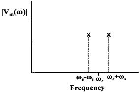
Vin(t) = Vs k/4R [cos(ωc + ωs)t + cos(ωc − ωs)t] |
(18) |
||||
This signal would have the magnitude spectrum given in Figure 8.11. This signal is termed a double side band suppressed-carrier modulation since the carrier frequency, ωc, is missing as seen in Figure 8.11.
FIGURE 8.11 Frequency spectrum of the signal created by sinusoidally exciting a variable resistance transducer with a carrier frequency ωc. This type of modulation is termed double sideband suppressed-carrier modulation since the carrier frequency is absent.
Copyright 2004 by Marcel Dekker, Inc. All Rights Reserved.
Note that using the identity:
cos(x) + cos(y) = 2 cos |
x + |
y |
cos |
x − |
y |
|
(19) |
2 |
|
2 |
|
||||
then Vin(t) can be written as: |
|
|
|
|
|
|
|
Vin(t) = Vs k/2R (cos(ωc t) cos(ωs t)) = A(t) cos(ωc t) |
(20) |
||||||
where |
|
|
|
|
|
|
|
A(t) = Vs k/2R (cos(ωcs t)) |
|
|
|
|
|
(21) |
|
Phase Sensitive Detectors
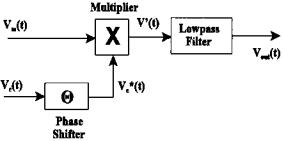
The basic configuration of a phase sensitive detector is shown in Figure 8.12 below. The first step in phase sensitive detection is multiplication by a phase shifted carrier.
Using the identity given in Eq. (18) the output of the multiplier, V ′(t), in Figure 8.12 becomes:
V′(t) = Vin(t) cos(ωc t + θ) = A(t) cos(ωc t) cos(ωc t + θ) |
|
= A(t)/2 [cos(2ωc t + θ) + cos θ] |
(22) |
To get the full spectrum, before filtering, substitute Eq. (21) for A(t) into Eq. (22):
V′(t) = Vs k/4R [cos(2ωc t + θ) cos(ωs t) + cos(ωs t) cos θ)] |
(23) |
again applying the identity in Eq. (17):
FIGURE 8.12 Basic elements and configuration of a phase sensitive detector used to demodulate AM signals.
Copyright 2004 by Marcel Dekker, Inc. All Rights Reserved.