Biosignal and Biomedical Image Processing MATLAB based Applications - John L. Semmlow

%Inputs

%x Complex signal

%fs Sample frequency

[N, xcol] = size(x);

%

%

%Compute instantaneous autocorrelation: Eq. (7) for ti = 1:N % Increment over time

taumax = min([ti-1,N-ti,round(N/2)-1]); tau = -taumax:taumax;

% Autocorrelation: tau is in columns and time is in rows WD(tau-tau(1) 1,ti) = x(ti tau) .* conj(x(ti-tau));

end

%

WD = fft(WD);

The last section of code is used to compute the instantaneous autocorrelation function and its Fourier transform as in Eq. (9c). The for loop is used to construct an array, WD, containing the instantaneous autocorrelation where each column contains the correlations at various lags for a given time, ti. Each column is computed over a range of lags, ± taumax. The first statement in the loop restricts the range of taumax to be within signal array: it uses all the data that is symmetrically available on either side of the time variable, ti. Note that the phase of the lag signal placed in array WD varies by column (i.e., time). Normally this will not matter since the Fourier transform will be taken over each set of lags (i.e., each column) and only the magnitude will be used. However, the phase was properly adjusted before plotting the instantaneous autocorrelation in Figure 6.1. After the instantaneous autocorrelation is constructed, the Fourier transform is taken over each set of lags. Note that if an array is presented to the MATLAB fft routine, it calculates the Fourier transform for each column; hence, the Fourier transform is computed for each value in time producing a two-dimensional function of time and frequency.

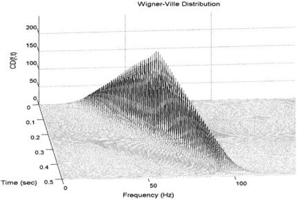
The Wigner-Ville is particularly effective at detecting single sinusoids that change in frequency with time, such as the chirp signal shown in Figure 6.5 and used in Example 6.2. For such signals, the Wigner-Ville distribution produces very few cross products, as shown in Example 6.4.

Copyright 2004 by Marcel Dekker, Inc. All Rights Reserved.

Example 6.4 Apply the Wigner-Ville distribution to a chirp signal the ranges linearly between 20 and 200 Hz over a 1 second time period. In this example, use the MATLAB chirp routine.

%Example 6.4 and Figure 6.9

%Example of the use of the Wigner-Ville distribution applied to

%a chirp

%Generates the chirp signal using the MATLAB chirp routine

%

clear all; close all; % Set up constants fs = 500;

N = 512; f1 = 20; f2 = 200;

%

% Construct “chirp” signal tn = (1:N)/fs;

FIGURE 6.9 Wigner-Ville of a chirp signal in which a single sine wave increases linearly with time. While both the time and frequency of the signal are welldefined, the amplitude, which should be constant, varies considerably.

Copyright 2004 by Marcel Dekker, Inc. All Rights Reserved.

.......3D labels, axis, view.......

If the analytic signal is not used, then the Wigner-Ville generates considerably more cross products. A demonstration of the advantages of using the analytic signal is given in Problem 2 at the end of the chapter.

Choi-Williams and Other Distributions

To implement other distributions in Cohen’s class, we will use the approach defined by Eq. (13). Following Eq. (13), the desired distribution can be obtained by convolving the related determining function (Eq. (17)) with the instantaneous autocorrelation function (Rx(t,τ); Eq. (7)) then taking the Fourier transform with respect to τ. As mentioned, this is simply a two-dimensional filtering of the instantaneous autocorrelation function by the appropriate filter (i.e., the determining function), in this case an exponential filter. Calculation of the instantaneous autocorrelation function has already been done as part of the Wigner-Ville calculation. To facilitate evaluation of the other distributions, we first extract the code for the instantaneous autocorrelation from the Wigner-Ville function, wvd in Example 6.3, and make it a separate function that can be used to determine the various distributions. This function has been termed int_autocorr, and takes the data as input and produces the instantaneous autocorrelation function as the output. These routines are available on the CD.

function Rx = int_autocorr(x)

%Function to compute the instantenous autocorrelation

%Output

%Rx instantaneous autocorrelation

%Input

%x signal

%

% Compute instantaneous autocorrelation for ti = 1:N % Increment over time

taumax = min([ti-1,N-ti,round(N/2)-1]); tau = -taumax:taumax;

Copyright 2004 by Marcel Dekker, Inc. All Rights Reserved.

Rx(tau-tau(1) 1,ti) = x(ti tau) .* conj(x(ti-tau));

end

The various members of Cohen’s class of distributions can now be implemented by a general routine that starts with the instantaneous autocorrelation function, evaluates the appropriate determining function, filters the instantaneous autocorrelation function by the determining function using convolution, then takes the Fourier transform of the result. The routine described below, cohen, takes the data, sample interval, and an argument that specifies the type of distribution desired and produces the distribution as an output along with time and frequency vectors useful for plotting. The routine is set up to evaluate four different distributions: Choi-Williams, Born-Jorden-Cohen, Rihaczek-Marge- nau, with the Wigner-Ville distribution as the default. The function also plots the selected determining function.

function [CD,f,t] = cohen(x,fs,type)

%Function to compute several of Cohen’s class of time–frequencey

%distributions

%

%Outputs

%CD Desired distribution

%f Frequency vector for plotting

%t Time vector for plotting %Inputs

%x Complex signal

% fs Sample frequency

%type of distribution. Valid arguements are:

%’choi’ (Choi-Williams), ’BJC’ (Born-Jorden-Cohen);

%and ’R_M’ (Rihaczek-Margenau) Default is Wigner-Ville

%Assign constants and check input

%

% Compute instantaneous autocorrelation: Eq. (7)

Copyright 2004 by Marcel Dekker, Inc. All Rights Reserved.

%Convolve determining function with instantaneous

%autocorrelation

CD = conv2(CD,G);

CD = CD(1:N,1:N);

%

% Take FFT again, FFT taken with respect to columns CD = flipud(fft(CD)); % Output distribution

The code to produce the Choi-Williams determining function is a straightforward implementation of G(t,τ) in Eq. (17) as shown below. The function is generated for only the first quadrant, then duplicated in the other quadrants. The function itself is plotted in Figure 6.10. The code for other determining functions follows the same general structure and can be found in the software accompanying this text.

function G = choi(sigma,N)

%Function to calculate the Choi-Williams distribution function

%(Eq. (17)

for i = 1:N/2

G(i,j) = exp(-(sigma*(i-1)v2)/(4*(j-1)v2)); wt = wt 2*G(i,j);

end

Copyright 2004 by Marcel Dekker, Inc. All Rights Reserved.

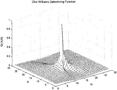
FIGURE 6.10 The Choi-Williams determining function generated by the code below.

G= [ fliplr(G(:,2:end)) G]; % Add 2nd quadrant

G= [flipud(G(2:end,:)); G]; % Add 3rd and 4th quadrants

To complete the package, Example 6.5 provides code that generates the data (either two sequential sinusoids or a chirp signal), asks for the desired distributions, evaluates the distribution using the function cohen, then plots the result. Note that the code for implementing Cohen’s class of distributions is written for educational purposes only. It is not very efficient, since many of the operations involve multiplication by zero (for example, see Figure 6.10 and Figure 6.11), and these operations should be eliminated in more efficient code.

Copyright 2004 by Marcel Dekker, Inc. All Rights Reserved.

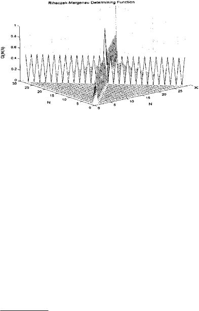
FIGURE 6.11 The determining function of the Rihaczek-Margenau distribution.

Example 6.5 Compare the Choi-Williams and Rihaczek-Margenau distributions for both a double sinusoid and chirp stimulus. Plot the RihaczekMargenau determining function* and the results using 3-D type plots.

%Example 6.5 and various figures

%Example of the use of Cohen’s class distributions applied to

%both sequential sinusoids and a chirp signal

%

clear all; close all; global G;

% Set up constants. (Same as in previous examples)

%

% Construct a step change in frequency

signal_type = input (’Signal type (1 = sines; 2 = chirp):’); if signal_type == 1

tn = (1:N/4)/fs;

x = [zeros(N/4,1); sin(2*pi*f1*tn)’; sin(2*pi*f2*tn)’;

*Note the code for the Rihaczek-Margenau determining function and several other determining functions can be found on disk with the software associated with this chapter.

Copyright 2004 by Marcel Dekker, Inc. All Rights Reserved.

zeros(N/4,1)]; else

tn = (1:N)/fs;

x = chirp(tn,f1,.5,f2)’; end

%

%

% Get desired distribution

type = input(’Enter type (choi,BJC,R_M,WV):’,’s’);

%

contour plot

xlabel(’Time (sec)’); ylabel(’Frequency (Hz)’); eval([’title(’,’heading’, ’);’]);

This program was used to generate Figures 6.11–6.15.

In this chapter we have explored only a few of the many possible time– frequency distributions, and, necessarily, covered only the very basics of this extensive subject. Two of the more important topics that were not covered here are the estimation of instantaneous frequency from the time–frequency distribution, and the effect of noise on these distributions. The latter is covered briefly in the problem set below.

PROBLEMS

1. Construct a chirp signal similar to that used in Example 6.2. Evaluate the analysis characteristics of the STFT using different window filters and sizes. Specifically, use window sizes of 128, 64, and 32 points. Repeat this analysis

Copyright 2004 by Marcel Dekker, Inc. All Rights Reserved.

FIGURE 6.12 Choi-Williams distribution for the two sequential sinusoids shown in Figure 6.3. Comparing this distribution with the Wigner-Ville distribution of the same stimulus, Figure 6.7, note the decreased cross product terms.

FIGURE 6.13 The Rihaczek-Margenau distribution for the sequential sinusoid signal. Note the very low value of cross products.

Copyright 2004 by Marcel Dekker, Inc. All Rights Reserved.

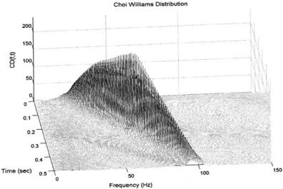
FIGURE 6.14 The Choi-Williams distribution from the chirp signal. Compared to the Wigner-Ville distribution (Figure 6.9), this distribution has a flatter ridge, but neither the Choi-Williams nor the the Wigner-Ville distributions show significant cross products to this type of signal.

using a Chebyshev window. (Modify spectog to apply the Chebyshev window, or else use MATLAB’s specgram.) Assume a sample frequency of 500 Hz and a total time of one second.

2.Rerun the two examples that involve the Wigner-Ville distribution (Examples 6.3 and 6.4), but use the real signal instead of the analytic signal. Plot the results as both 3-D mesh plots and contour plots.

3.Construct a signal consisting of two components: a continuous sine wave of 20 Hz and a chirp signal that varies from 20 Hz to 100 Hz over a 0.5 sec time period. Analyze this signal using two different distributions: Wigner-Ville and Choi-Williams. Assume a sample frequency of 500 Hz, and use analytical signal.

4.Repeat Problem 3 above using the Born-Jordan-Cohen and RihaczekMargenau distributions.

5.Construct a signal consisting of two sine waves of 20 and 100 Hz. Add to this signal Gaussian random noise having a variance equal to 1/4 the amplitude of the sinusoids. Analyze this signal using the Wigner-Ville and Choi-Williams

Copyright 2004 by Marcel Dekker, Inc. All Rights Reserved.