Biosignal and Biomedical Image Processing MATLAB based Applications - John L. Semmlow

the sidelobes. Most alternatives to the rectangular window reduce the sidelobes (they decay away more quickly than those of Figure 3.6), but at the cost of wider mainlobes. Figures 3.7 and 3.8 show the shape and frequency spectra produced by two popular windows: the triangular window and the raised cosine or Hamming window. The algorithms for these windows are straightforward:

Triangular window: for odd n:

FIGURE 3.7 The triangular window in the time domain (left) and its spectral characteristic (right). The sidelobes diminish faster than those of the rectangular window (Figure 3.6), but the mainlobe is wider.

Copyright 2004 by Marcel Dekker, Inc. All Rights Reserved.

FIGURE 3.8 The Hamming window in the time domain (left) and its spectral characteristic (right).

These and several others are easily implemented in MATLAB, especially with the Signal Processing Toolbox as described in the next section. A MATLAB routine is also described to plot the spectral characteristics of these and other windows. Selecting the appropriate window, like so many other aspects of signal analysis, depends on what spectral features are of interest. If the task is to resolve two narrowband signals closely spaced in frequency, then a window with the narrowest mainlobe (the rectangular window) is preferred. If there is a strong and a weak signal spaced a moderate distance apart, then a window with rapidly decaying sidelobes is preferred to prevent the sidelobes of the strong signal from overpowering the weak signal. If there are two moderate strength signals, one close and the other more distant from a weak signal, then a compromise window with a moderately narrow mainlobe and a moderate decay in sidelobes could be the best choice. Often the most appropriate window is selected by trial and error.

Power Spectrum

The power spectrum is commonly defined as the Fourier transform of the autocorrelation function. In continuous and discrete notation, the power spectrum equation becomes:

Copyright 2004 by Marcel Dekker, Inc. All Rights Reserved.

T

PS(f) = ∫ rxx(τ) e−2πf T τ dτ

0

N−1

n=0

where rxx(n) is the autocorrelation function described in Chapter 2. Since the autocorrelation function has odd symmetry, the sine terms, b(k) will all be zero (see Table 3.1) and Eq. (14) can be simplified to include only real cosine terms.

T

PS(f) = ∫ rxx(τ) cos(2πmfT t) dτ

n=0

These equations in continuous and discrete form are sometimes referred to as the cosine transform. This approach to evaluating the power spectrum has lost favor to the so-called direct approach, given by Eq. (18) below, primarily because of the efficiency of the fast Fourier transform. However, a variation of this approach is used in certain time–frequency methods described in Chapter 6. One of the problems compares the power spectrum obtained using the direct approach of Eq. (18) with the traditional method represented by Eq. (14).

The direct approach is motivated by the fact that the energy contained in an analog signal, x(t), is related to the magnitude of the signal squared, integrated over time:

−∞

By an extension of Parseval’s theorem it is easy to show that:

Hence *X( f )*2 equals the energy density function over frequency, also referred to as the energy spectral density, the power spectral density, or simply the power spectrum. In the direct approach, the power spectrum is calculated as the magnitude squared of the Fourier transform of the waveform of interest:

Power spectral analysis is commonly applied to truncated data, particularly when the data contains some noise, since phase information is less useful in such situations.

Copyright 2004 by Marcel Dekker, Inc. All Rights Reserved.

While the power spectrum can be evaluated by applying the FFT to the entire waveform, averaging is often used, particularly when the available waveform is only a sample of a longer signal. In such very common situations, power spectrum evaluation is necessarily an estimation process, and averaging improves the statistical properties of the result. When the power spectrum is based on a direct application of the Fourier transform followed by averaging, it is commonly referred to as an average periodogram. As with the Fourier transform, evaluation of power spectra involves necessary trade-offs to produce statistically reliable spectral estimates that also have high resolution. These trade-offs are implemented through the selection of the data window and the averaging strategy. In practice, the selection of data window and averaging strategy is usually based on experimentation with the actual data.

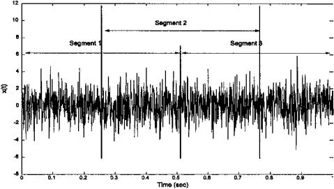
Considerations regarding data windowing have already been described and apply similarly to power spectral analysis. Averaging is usually achieved by dividing the waveform into a number of segments, possibly overlapping, and evaluating the Fourier transform on each of these segments (Figure 3.9). The final spectrum is taken from an average of the Fourier transforms obtained from the various segments. Segmentation necessarily reduces the number of data sam-

FIGURE 3.9 A waveform is divided into three segments with a 50% overlap between each segment. In the Welch method of spectral analysis, the Fourier transform of each segment would be computed separately, and an average of the three transforms would provide the output.

Copyright 2004 by Marcel Dekker, Inc. All Rights Reserved.

ples evaluated by the Fourier transform in each segment. As mentioned above, frequency resolution of a spectrum is approximately equal to 1/NTs, where N is now the number samples per segment. Choosing a short segment length (a small N ) will provide more segments for averaging and improve the reliability of the spectral estimate, but it will also decrease frequency resolution. Figure 3.2 shows spectra obtained from a 1024-point data array consisting of a 100 Hz sinusoid and white noise. In Figure 3.2A, the periodogram is taken from the entire waveform, while in Figure 3.2B the waveform is divided into 32 nonoverlapping segments; a Fourier transform is calculated from each segment, then averaged. The periodogram produced from the segmented and averaged data is much smoother, but the loss in frequency resolution is apparent as the 100 Hz sine wave is no longer visible.

One of the most popular procedures to evaluate the average periodogram is attributed to Welch and is a modification of the segmentation scheme originally developed by Bartlett. In this approach, overlapping segments are used, and a window is applied to each segment. By overlapping segments, more segments can be averaged for a given segment and data length. Averaged periodograms obtained from noisy data traditionally average spectra from half-overlap- ping segments; that is, segments that overlap by 50%. Higher amounts of overlap have been recommended in other applications, and, when computing time is not factor, maximum overlap has been recommended. Maximum overlap means shifting over by just a single sample to get the new segment. Examples of this approach are provided in the next section on implementation.

The use of data windowing for sidelobe control is not as important when the spectra are expected to be relatively flat. In fact, some studies claim that data windows give some data samples more importance than others and serve only to decrease frequency resolution without a significant reduction in estimation error. While these claims may be true for periodograms produced using all the data (i.e., no averaging), they are not true for the Welch periodograms because overlapping segments serves to equalize data treatment and the increased number of segments decreases estimation errors. In addition, windows should be applied whenever the spectra are expected have large amplitude differences.

MATLAB IMPLEMENTATION

Direct FFT and Windowing

MATLAB provides a variety of methods for calculating spectra, particularly if the Signal Processing Toolbox is available. The basic Fourier transform routine is implemented as:

X = fft(x,n)

Copyright 2004 by Marcel Dekker, Inc. All Rights Reserved.

where X is the input waveform and x is a complex vector providing the sinusoidal coefficients. The argument n is optional and is used to modify the length of data analyzed: if n < length(x), then the analysis is performed over the first n points; or, if n > length(x), x is padded with trailing zeros to equal n. The fft routine implements Eq. (6) above and employs a high-speed algorithm. Calculation time is highly dependent on data length and is fastest if the data length is a power of two, or if the length has many prime factors. For example, on one machine a 4096-point FFT takes 2.1 seconds, but requires 7 seconds if the sequence is 4095 points long, and 58 seconds if the sequence is for 4097 points. If at all possible, it is best to stick with data lengths that are powers of two.

The magnitude of the frequency spectra can be easily obtained by applying the absolute value function, abs, to the complex output X:

Magnitude = abs(X)

This MATLAB function simply takes the square root of the sum of the real part of X squared and the imaginary part of X squared. The phase angle of the spectra can be obtained by application of the MATLAB angle function:

Phase = angle(X)

The angle function takes the arctangent of the imaginary part divided by the real part of Y. The magnitude and phase of the spectrum can then be plotted using standard MATLAB plotting routines. An example applying the MATLAB fft to a array containing sinusoids and white noise is provided below and the resultant spectra is given in Figure 3.10. Other applications are explored in the problem set at the end of this chapter. This example uses a special routine, sig_noise, found on the disk. The routine generates data consisting of sinusoids and noise that are useful in evaluating spectral analysis algorithms. The calling structure for sig_noise is:

[x,t] = sig_noise([f],[SNR],N);

where f specifies the frequency of the sinusoid(s) in Hz, SNR specifies the desired noise associated with the sinusoid(s) in db, and N is the number of points. The routine assumes a sample frequency of 1 kHz. If f and SNR are vectors, multiple sinusoids are generated. The output waveform is in x and t is a time vector useful in plotting.

Example 3.1 Plot the power spectrum of a waveform consisting of a single sine wave and white noise with an SNR of −7 db.

Copyright 2004 by Marcel Dekker, Inc. All Rights Reserved.

FIGURE 3.10 Plot produced by the MATLAB program above. The peak at 250 Hz is apparent. The sampling frequency of this data is 1 kHz, hence the spectrum is symmetric about the Nyquist frequency, fs/2 (500 Hz). Normally only the first half of this spectrum would be plotted (SNR = −7 db; N = 1024).

%Example 3.1 and Figure 3.10 Determine the power spectrum

%of a noisy waveform

%First generates a waveform consisting of a single sine in

%noise, then calculates the power spectrum from the FFT

%and plots

%Generate data using sig_noise

%250 Hz sin plus white noise; N data points ; SNR = -7 db [x,t] = sig_noise (250,-7,N);

fs = 1000;

Y = fft(x);

PS = abs(Y).v2;

Copyright 2004 by Marcel Dekker, Inc. All Rights Reserved.

title(’Power Spectrum (note symmetric about fs/2)’); xlabel(’Frequency (Hz)’);

ylabel(’Power Spectrum (db)’);

The Welch Method for Power Spectral

Density Determination

As described above, the Welch method for evaluating the power spectrum divides the data in several segments, possibly overlapping, performs an FFT on each segment, computes the magnitude squared (i.e., power spectrum), then averages these spectra. Coding these in MATLAB is straightforward, but this is unnecessary as the Signal Processing Toolbox features a function that performs these operations. In its more general form, the pwelch* function is called as:

[PS,f] = pwelch(x,window,noverlap,nfft,fs)

Only the first input argument, the name of the data vector, is required as the other arguments have default values. By default, x is divided into eight sections with 50% overlap, each section is windowed with a Hamming window and eight periodograms are computed and averaged. If window is an integer, it specifies the segment length, and a Hamming window of that length is applied to each segment. If window is a vector, then it is assumed to contain the window function (easily implemented using the window routines described below). In this situation, the window size will be equal to the length of the vector, usually set to be the same as nfft. If the window length is specified to be less than nfft (greater is not allowed), then the window is zero padded to have a length equal to nfft. The argument noverlap specifies the overlap in samples. The sampling frequency is specified by the optional argument fs and is used to fill the frequency vector, f, in the output with appropriate values. This output variable can be used in plotting to obtain a correctly scaled frequency axis (see Example 3.2). As is always the case in MATLAB, any variable can be omitted, and the default selected by entering an empty vector, [ ].

If pwelch is called with no output arguments, the default is to plot the power spectral estimate in dB per unit frequency in the current figure window. If PS is specified, then it contains the power spectra. PS is only half the length of the data vector, x, specifically, either (nfft/2) 1 if nfft is even, or (nfft 1)/2 for nfft odd, since the additional points would be redundant. (An

*The calling structure for this function is different in MATLAB versions less than 6.1. Use the ‘Help’ command to determine the calling structure if you are using an older version of MATLAB.

Copyright 2004 by Marcel Dekker, Inc. All Rights Reserved.

exception is made if x is complex data in which case the length of PS is equal to nfft.) Other options are available and can be found in the help file for pwelch.

Example 3.2 Apply Welch’s method to the sine plus noise data used in Example 3.1. Use 124-point data segments and a 50% overlap.

%Example 3.2 and Figure 3.11

%Apply Welch’s method to sin plus noise data of Figure 3.10 clear all; close all;

N = 1024; fs = 1000;

FIGURE 3.11 The application of the Welch power spectral method to data containing a single sine wave plus noise, the same as the one used to produce the spectrum of Figure 3.10. The segment length was 128 points and segments overlapped by 50%. A triangular window was applied. The improvement in the background spectra is obvious, although the 250 Hz peak is now broader.

Copyright 2004 by Marcel Dekker, Inc. All Rights Reserved.

%Generate data (250 Hz sin plus noise) [x,t,] = sig_noise(250,-7,N);

%Estimate the Welch spectrum using 128 point segments,

%a the triangular filter, and a 50% overlap.

%

[PS,f] = (x, triang(128),[ ],128,fs); plot(f,PS,’k’); % Plot power spectrum title(’Power Spectrum (Welch Method)’); xlabel(’Frequency (Hz)’);

ylabel(’Power Spectrum’);

Comparing the spectra in Figure 3.11 with that of Figure 3.10 shows that the background noise is considerably smoother and reduced. The sine wave at 250 Hz is clearly seen, but the peak is now slightly broader indicating a loss in frequency resolution.

Window Functions

MATLAB has a number of data windows available including those described in Eqs. (11–13). The relevant MATLAB routine generates an n-point vector array containing the appropriate window shape. All have the same form:

where N is the number of points in the output vector and window_name is the name, or an abbreviation of the name, of the desired window. At this writing, thirteen different windows are available in addition to rectangular (rectwin) which is included for completeness. Using help window will provide a list of window names. A few of the more popular windows are: bartlett, blackman, gausswin, hamming (a common MATLAB default window), hann, kaiser, and triang. A few of the routines have additional optional arguments. In particular, chebwin (Chebyshev window), which features a nondecaying, constant level of sidelobes, has a second argument to specify the sidelobe amplitude. Of course, the smaller this level is set, the wider the mainlobe, and the poorer the frequency resolution. Details for any given window can be found through the help command. In addition to the individual functions, all of the window functions can be constructed with one call:

w = window(@name,N,opt) % Get N-point window ‘name.’

Copyright 2004 by Marcel Dekker, Inc. All Rights Reserved.