Biosignal and Biomedical Image Processing MATLAB based Applications - John L. Semmlow

MATLAB Implementation

Of the techniques described above, only the Hough transform is supported by MATLAB image processing routines, and then only for straight lines. It is supported as the Radon transform which computes projections of the image along a straight line, but this projection can be done at any angle.* This results in a projection matrix that is the same as the accumulator array for a straight line Hough transform when expressed in cylindrical coordinates.

The Radon transform is implemented by the statement:

[R, xp] = radon(BW, theta);

where BW is a binary input image and theta is the projection angle in degrees, usually a vector of angles. If not specified, theta defaults to (1:179). R is the projection array where each column is the projection at a specific angle. (R is a column vector if theta is a constant). Hence, maxima in R correspond to the positions (encoded as an angle and distance) in the image. An example of the use of radon to perform the Hough transformation is given in Example 12.7.

Example 12.7 Find the strongest line in the image of Saturn in image file ‘saturn.tif’. Plot that line superimposed on the image.

Solution First convert the image to an edge array using MATLAB’s edge routine. Use the Hough transform (implemented for straight lines using radon) to build an accumulator array. Find the maximum point in that array (using max) which will give theta, the angle perpendicular to the line, and the distance along that perpendicular line of the intersection. Convert that line to rectangular coordinates, then plot the line superimposed on the image.

%Example 12.7 Example of the Hough transform

%(implemented using ‘radon’) to identify lines in an image.

%Use the image of Saturn in ‘saturn.tif’

% Convert to indexed image

[X, map] = gray2ind (mat2gray(R));

*The Radon transform is an important concept in computed tomography (CT) as described in a following section.

Copyright 2004 by Marcel Dekker, Inc. All Rights Reserved.

%

subplot(1,2,1); imshow(BW) % Display results title(‘Saturn Thresholded’);

subplot(1,2,2); imshow(X, hot);

% The hot colormap gives better % reproduction

b= -r/cos((c-90)*radians); % Intercept from basic

%trigonometry

This example produces the images shown in Figure 12.20. The broad white line superimposed is the line found as the most dominant using the Hough transform. The location of this in the accumulator or parameter space array is shown in the right-hand image. Other points nearly as strong (i.e., bright) can be seen in the parameter array which represent other lines in the image. Of course, it is possible to identify these lines as well by searching for maxima other than the global maximum. This is done in a problem below.

PROBLEMS

1.Load the blood cell image (blood1.tif) Filter the image with two lowpass

filters, one having a weak cutoff (for example, Gaussian with an alpha of 0.5) and the other having a strong cutoff (alpha > 4). Threshold the two filtered images using the maximum variance routine (graythresh). Display the original and filtered images along with their histograms. Also display the thresholded images.

2.The Laplacian filter which calculates the second derivative can also be used to find edges. In this case edges will be located where the second derivative is near zero. Load the image of the spine (‘spine.tif’) and filter using the Laplacian filter (use the default constant). Then threshold this image using

Copyright 2004 by Marcel Dekker, Inc. All Rights Reserved.

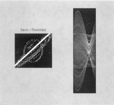
FIGURE 12.20 Thresholded image of Saturn (from MATLAB’s saturn.tif) with the dominant line found by the Hough transform. The right image is the accumulator array with the maximum point indicated by an ‘*’. (Original image is a public domain image courtesy of NASA, Voyger 2 image, 1981-08-24.)

islice. The threshold values should be on either side of zero and should be quite small (< 0.02) since you are interested in values quite close to zero.

3. Load image ‘texture3.tif’ which contains three regions having the same average intensities but different textural patterns. Before applying the nonlinear range operator used in Example 12.2, preprocess with a Laplacian filter (alpha = 0.5). Apply the range operator as in Example 12.2 using nlfilter. Plot original and range images along with their histograms. Threshold the range image to isolate the segments and compare with the figures in the book. (Hint: You may have to adjust the thresholds slightly, but you do not have to rerun the timeconsuming range operator to adjust these thresholds.) You should observe a modest improvement: one of the segments can now be perfectly separated.

Copyright 2004 by Marcel Dekker, Inc. All Rights Reserved.

4.Load the texture orientation image texture4.tif. Separate the segments as well as possible by using a Sobel operator followed by a standard deviation operator implemented using nlfilter. (Note you will have to multiply the standard deviation image by around 4 to get it into an appropriate range.) Plot the histogram and use it to determine the best boundaries for separating the three segments. Display the three segments as white objects.

5.Load the thresholded image of Figure 12.5 (found as Fig12_5.tif on the disk) and use opening to eliminate as many points as possible in the upper field without affecting the lower field. Then use closing to try to blacken as many points as possible in the lower field without affecting the upper field. (You should be able to blacken the lower field completely except for edge effects.)

Copyright 2004 by Marcel Dekker, Inc. All Rights Reserved.

13

Image Reconstruction

Medical imaging utilizes several different physical principals or imaging modalities. Common modalities used clinically include x-ray, computed tomography (CT), positron emission tomography (PET), single photon emission computed tomography (SPECT), and ultrasound. Other approaches under development include optical imaging* and impedence tomography. Except for simple x-ray images which provide a shadow of intervening structures, some form of image processing is required to produce a useful image. The algorithms used for image reconstruction depend on the modality. In magnetic resonance imaging (MRI), reconstruction techniques are fairly straightforward, requiring only a two-dimen- sional inverse Fourier transform (described later in this chapter). Positron emission tomography (PET) and computed tomography use projections from collimated beams and the reconstruction algorithm is critical. The quality of the image is strongly dependent on the image reconstruction algorithm.†

*Of course, optical imaging is used in microscopy, but because of scattering it presents serious problems when deep tissues are imaged. A number of advanced image processing methods are under development to overcome problems due to scattering and provide useful images using either coherent or noncoherent light.

†CT may be the first instance where the analysis software is an essential component of medical diagnosis and comes between the physician and patient: the physician has no recourse but to trust the software.

Copyright 2004 by Marcel Dekker, Inc. All Rights Reserved.

CT, PET, AND SPECT

Reconstructed images from PET, SPECT, and CT all use collimated beams directed through the target, but they vary in the mechanism used to produce these collimated beams. CT is based on x-ray beams produced by an external source that are collimated by the detector: the detector includes a collimator, usually a long tube that absorbs diagonal or off-axis photons. A similar approach is used for SPECT, but here the photons are produced by the decay of a radioactive isotope within the patient. Because of the nature of the source, the beams are not as well collimated in SPECT, and this leads to an unavoidable reduction in image resolution. Although PET is also based on photons emitted from a radioactive isotope, the underlying physics provide an opportunity to improve beam collimation through so-called electronic collimation. In PET, the radioactive isotope emits a positron. Positrons are short lived, and after traveling only a short distance, they interact with an electron. During this interaction, their masses are annihilated and two photons are generated traveling in opposite directions, 180 deg. from one another. If two separate detectors are activated at essentially the same time, then it is likely a positron annihilation occurred somewhere along a line connecting these two detectors. This coincident detection provides an electronic mechanism for establishing a collimated path that traverses the original positron emission. Note that since the positron does not decay immediately, but may travel several cm in any direction before annihilation, there is an inherent limitation on resolution.

In all three modalities, the basic data consists of measurements of the absorption of x-rays (CT) or concentrations of radioactive material (PET and SPECT), along a known beam path. From this basic information, the reconstruction algorithm must generate an image of either the tissue absorption characteristics or isotope concentrations. The mathematics are fairly similar for both absorption and emission processes and will be described here in terms of absorption processes; i.e., CT. (See Kak and Slaney (1988) for a mathematical description of emission processes.)

In CT, the intensity of an x-ray beam is dependent on the intensity of the source, Io, the absorption coefficient, µ, and length, R, of the intervening tissue:

where I(x,y) is the beam intensity (proportional to number of photons) at position x,y. If the beam passes through tissue components having different absorption coefficients then, assuming the tissue is divided into equal sections ∆R, Eq.

(1) becomes:

Copyright 2004 by Marcel Dekker, Inc. All Rights Reserved.

The projection p(x,y), is the log of the intensity ratio, and is obtained by dividing out Io and taking the natural log:

Eq. (3) is also expressed as a continuous equation where it becomes the line integral of the attenuation coefficients from the source to the detector:

Source

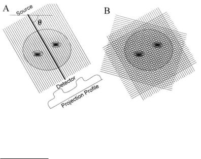
Figure 13.1A shows a series of collimated parallel beams traveling through tissue.* All of these beams are at the same angle, θ, with respect to the reference axis. The output of each beam is just the projection of absorption characteristics of the intervening tissue as defined in Eq. (4). The projections of all the individual parallel beams constitute a projection profile of the intervening

FIGURE 13.1 (A) A series of parallel beam paths at a given angle, θ, is projected through biological tissue. The net absorption of each beam can be plotted as a projection profile. (B) A large number of such parallel paths, each at a different angle, is required to obtain enough information to reconstruct the image.

*In modern CT scanners, the beams are not parallel, but dispersed in a spreading pattern from a single source to an array of detectors, a so-called fan beam pattern. To simplify the analysis presented here, we will assume a parallel beam geometry. Kak and Slaney (1988) also cover the derivation of reconstruction algorithms for fan beam geometry.

Copyright 2004 by Marcel Dekker, Inc. All Rights Reserved.

tissue absorption coefficients. With only one projection profile, it is not possible to determine how the tissue absorptions are distributed along the paths. However, if a large number of projections are taken at different angles through the tissue, Figure 13.1B, it ought to be possible, at least in principle, to estimate the distribution of absorption coefficients from some combined analysis applied to all of the projections. This analysis is the challenge given to the CT reconstruction algorithm.

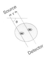
If the problem were reversed, that is, if the distribution of tissue absorption coefficients was known, determining the projection profile produced by a set of parallel beams would be straightforward. As stated in Eq. (13-4), the output of each beam is the line integral over the beam path through the tissue. If the beam is at an angle, θ (Figure 13-2), then the equation for a line passing through the origin at angle θ is:

where I(x,y) is the distribution of absorption coefficients as Eq. (2). If the beam is displaced a distance, r, from the axis in a direction perpendicular to θ, Figure 13.2, the equation for that path is:

FIGURE 13.2 A single beam path is defined mathematically by the equation given in Eq. (5).

Copyright 2004 by Marcel Dekker, Inc. All Rights Reserved.

The whole family of parallel paths can be mathematically defined using Eqs. (6) and (7) combined with the Dirac delta distribution, δ, to represent the discrete parallel beams. The equation describing the entire projection profile, pθ(r), becomes:

This equation is known as the Radon transform, . It is the same as the Hough transform (Chapter 12) for the case of straight lines. The expression for pθ(r) can also be written succinctly as:

The forward Radon transform can be used to generate raw CT data from image data, useful in problems, examples, and simulations. This is the approach that is used in some of the examples given in the MATLAB Implementation section, and also to generate the CT data used in the problems.

The Radon transform is helpful in understanding the problem, but does not help in the actual reconstruction. Reconstructing the image from the projection profiles is a classic inverse problem. You know what comes out—the projection profiles—but want to know the image (or, in the more general case, the system), that produced that output. From the definition of the Radon transform in Eq. (9), the image should result from the application of an inverse Radon transform −1, to the projection profiles, pθ(r):

While the Radon transform (Eqs. (8) and (9)) and inverse Radon transform (Eq. (10)) are expressed in terms of continuous variables, in imaging systems the absorption coefficients are given in terms of discrete pixels, I(n,m), and the integrals in the above equations become summations. In the discrete situation, the absorption of each pixel is an unknown, and each beam path provides a single projection ratio that is the solution to a multi-variable equation. If the image contains N by M pixels, and there are N × M different projections (beam paths) available, then the system is adequately determined, and the reconstruction problem is simply a matter of solving a large number of simultaneous equations. Unfortunately, the number of simultaneous equations that must be solved is generally so large that a direct solution becomes unworkable. The early attempts at CT reconstruction used an iterative approach called the algebraic reconstruction algorithm or ART. In this algorithm, each pixel was updated based on errors between projections that would be obtained from the current pixel values and the actual projections. When many pixels are involved, conver-

Copyright 2004 by Marcel Dekker, Inc. All Rights Reserved.

gence was slow and the algorithm was computationally intensive and timeconsuming. Current approaches can be classified as either transform methods or series expansion methods. The filtered back-projection method described below falls into the first category and is one of the most popular of CT reconstruction approaches.

Filtered back-projection can be described in either the spatial or spatial frequency domain. While often implemented in the latter, the former is more intuitive. In back-projection, each pixel absorption coefficient is set to the sum (or average) of the values of all projections that traverse the pixel. In other words, each projection that traverses a pixel contributes its full value to the pixel, and the contributions from all of the beam paths that traverse that pixel are simply added or averaged. Figure 13.3 shows a simple 3-by-3 pixel grid with a highly absorbing center pixel (absorption coefficient of 8) against a background of lessor absorbing pixels. Three projection profiles are shown traversing the grid horizontally, vertically, and diagonally. The lower grid shows the image that would be reconstructed using back-projection alone. Each grid contains the average of the projections though that pixel. This reconstructed image resembles the original with a large central value surrounded by smaller values, but the background is no longer constant. This background variation is the result of blurring or smearing the central image over the background.

To correct the blurring or smoothing associated with the back-projection method, a spatial filter can be used. Since the distortion is in the form of a blurring or smoothing, spatial differentiation is appropriate. The most common filter is a pure derivative up to some maximum spatial frequency. In the frequency domain, this filter, termed the Ram-Lak filter, is a ramp up to some maximum cutoff frequency. As with all derivative filters, high-frequency noise will be increased, so this filter is often modified by the addition of a lowpass filter. Lowpass filters that can be used include the Hamming window, the Hanning window, a cosine window, or a sinc function window (the Shepp-Logan filter). (The frequency characteristics of these filters are shown in Figure 13.4). Figure 13.5 shows a simple image of a light square on a dark background. The projection profiles produced by the image are also shown (calculated using the Radon transform).

The back-projection reconstruction of this image shows a blurred version of the basic square form with indistinct borders. Application of a highpass filter sharpens the image (Figure 13.4). The MATLAB implementation of the inverse Radon transform, iradon described in the next section, uses the filtered backprojection method and also provides for all of the filter options.

Filtered back-projection is easiest to implement in the frequency domain. The Fourier slice theorem states that the one-dimensional Fourier transform of a projection profile forms a single, radial line in the two-dimensional Fourier transform of the image. This radial line will have the same angle in the spatial

Copyright 2004 by Marcel Dekker, Inc. All Rights Reserved.