Biosignal and Biomedical Image Processing MATLAB based Applications - John L. Semmlow

%Generate a single horizontal line of the image in a vector of

%400 points

%

% Generate sin; scale between 0&1 I_sin(1,:) = .5 * sin(2*pi*x) .5;

title(’Sinewave Grating’);

The output of this example is shown as Figure 10.3. As with all images shown in this text, there is a loss in both detail (resolution) and grayscale variation due to losses in reproduction. To get the best images, these figures, and all figures in this section can be reconstructed on screen using the code from the examples provided in the CD.

Example 10.2 Generate a multiframe variable consisting of a series of sinewave gratings having different phases. Display these images as a montage. Border the images with black for separation on the montage plot. Generate 12 frames, but reduce the image to 100 by 100 to save memory.

%Example 10.2 and Figure 10.4

%Generate a multiframe array consisting of sinewave gratings

%that vary in phase from 0 to 2 * pi across 12 images

%

%The gratings should be the same as in Example 10.1 except with

%fewer pixels (100 by 100) to conserve memory.

Copyright 2004 by Marcel Dekker, Inc. All Rights Reserved.

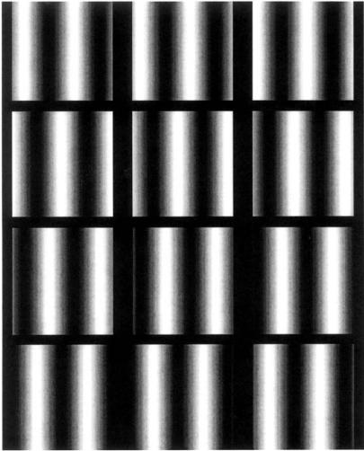
FIGURE 10.4 Montage of sinewave gratings created by Example 10.2.

Copyright 2004 by Marcel Dekker, Inc. All Rights Reserved.

I(i,:,1,j) = I_8;

end

end

end

title(’Sinewave Grating’);

The montage created by this example is shown in Figure 10.4 on the next page. The multiframe data set was constructed one frame at a time and the frame was placed in I using the frame index, the fourth index of I.* Zeros are inserted at the beginning and end of the sinewave and, in the image construction loop, for the first and last 9 points. This is to provide a dark band between the images. Finally the sinewave was phase shifted through 360 degrees over the 12 frames.

Example 10.3 Construct a multiframe variable with 12 sinewave grating images. Display these data as a movie. Since the immovie function requires the multiframe image variable to be in either RGB or indexed format, convert the uint16 data to indexed format. This can be done by the gray2ind(I,N) function. This function simply scales the data to be between 0 and N, where N is the depth of the colormap. If N is unspecified, gray2ind defaults to 64 levels. MATLAB colormaps can also be specified to be of any depth, but as with gray2ind the default level is 64.

%Example 10.3

%Generate a movie of a multiframe array consisting of sinewave

%gratings that vary in phase from 0 to pi across 10 images

%Since function ’immovie’ requires either RGB or indexed data

%formats scale the data for use as Indexed with 64 gray levels.

%Use a standard MATLAB grayscale (’gray’);

%

%The gratings should be the same as in Example 10.2.

clear all; close all;

%Assign parameters

N = 100;

Nu_cyc = 2;

M = 12;

%

x = (1:N)*Nu_cyc/N;

*Recall, the third index is reserved for referencing the color plane. For non-RGB variables, this index will always be 1. For images in RGB format the third index would vary between 1 and 3.

Copyright 2004 by Marcel Dekker, Inc. All Rights Reserved.

To fully appreciate this example, the reader will need to run this program under MATLAB. The 12 frames are created as in Example 10.3, except the code that adds border was removed and the data scaling was added. The second argument in immovie, is the colormap matrix and this example uses the map generated by gray2ind. This map has the default level of 64, the same as all of the other MATLAB supplied colormaps. Other standard maps that are appropriate for grayscale images are ‘bone’ which has a slightly bluish tint, ‘pink’ which has a decidedly pinkish tint, and ‘copper’ which has a strong rust tint. Of course any colormap can be used, often producing interesting pseudocolor effects from grayscale data. For an interesting color alternative, try running Example 10.3 using the prepackaged colormap jet as the second argument of immovie. Finally, note that the size of the multiframe array, Mf, is (100,100,1,12) or 1.2 × 105 × 2 bytes. The variable mov generated by immovie is even larger!

Image Storage and Retrieval

Images may be stored on disk using the imwrite command:

imwrite(I, filename.ext, arg1, arg2, ...);

where I is the array to be written into file filename. There are a large variety of file formats for storing image data and MATLAB supports the most popular formats. The file format is indicated by the filename’s extension, ext, which may be:

.bmp (Microsoft bitmap), .gif (graphic interchange format), .jpeg (Joint photographic experts group), .pcs (Paintbrush), .png (portable network graphics), and

.tif (tagged image file format). The arguments are optional and may be used to specify image compression or resolution, or other format dependent information.

Copyright 2004 by Marcel Dekker, Inc. All Rights Reserved.

The specifics can be found in the imwrite help file. The imwrite routine can be used to store any of the data formats or data classes mentioned above; however, if the data array, I, is an indexed array, then it must be followed by the colormap variable, map. Most image formats actually store uint8 formatted data, but the necessary conversions are done by the imwrite.

The imread function is used to retrieve images from disk. It has the calling structure:

[I map] = imread(‘filename.ext’,fmt or frame);

where filename is the name of the image file and .ext is any of the extensions listed above. The optional second argument, fmt, only needs to be specified if the file format is not evident from the filename. The alternative optional argument frame is used to specify which frame of a multiframe image is to be read in I. An example that reads multiframe data is found in Example 10.4. As most file formats store images in uint8 format, I will often be in that format. File formats .tif and .png support uint16 format, so imread may generate data arrays in uint16 format for these file types. The output class depends on the manner in which the data is stored in the file. If the file contains a grayscale image data, then the output is encoded as an intensity image, if truecolor, then as RGB. For both these cases the variable map will be empty, which can be checked with the isempty(map) command (see Example 10.4). If the file contains indexed data, then both output, I and map will contain data.

The type of data format used by a file can also be obtained by querying a graphics file using the function infinfo.

information = infinfo(‘filename.ext’)

where information will contain text providing the essential information about the file including the ColorType, FileSize, and BitDepth. Alternatively, the image data and map can be loaded using imread and the format image data determined from the MATLAB whos command. The whos command will also give the structure of the data variable (uint8, uint16, or double).

Basic Arithmetic Operations

If the image data are stored in the double format, then all MATLAB standard mathematical and operational procedures can be applied directly to the image variables. However, the double format requires 4 times as much memory as the uint16 format and 8 times as much memory as the uint8 format. To reduce the reliance on the double format, MATLAB has supplied functions to carry out some basic mathematics on uint8and uint16-format arrays. These routines will work on either format; they actually carry out the operations in double precision

Copyright 2004 by Marcel Dekker, Inc. All Rights Reserved.

on an element by element basis then convert back to the input format. This reduces roundoff and overflow errors. The basic arithmetic commands are:

For the last four routines, J can be either another image variable, or a constant. Several arithmetical operations can be combined using the imlincomb function. The function essentially calculates a weighted sum of images. For example to add 0.5 of image I1 to 0.3 of image I2, to 0.75 of Image I3, use:

% Linear combination of images

I_combined = imlincomb (.5, I1, .3, I2, .75, I3);

The arithmetic operations of multiplication and addition by constants are easy methods for increasing the contrast or brightness or an image. Some of these arithmetic operations are illustrated in Example 10.4.

Example 10.4 This example uses a number of the functions described previously. The program first loads a set of MRI (magnetic resonance imaging) images of the brain from the MATLAB Image Processing Toolbox’s set of stock images. This image is actually a multiframe image consisting of 27 frames as can be determined from the command imifinfo. One of these frames is selected by the operator and this image is then manipulated in several ways: the contrast is increased; it is inverted; it is sliced into 5 levels (N_slice); it is modified horizontally and vertically by a Hanning window function, and it is thresholded and converted to a binary image.

%Example 10.4 and Figures 10.5 and 10.6

%Demonstration of various image functions.

%Load all frames of the MRI image in mri.tif from the the MATLAB

%Image Processing Toolbox (in subdirectory imdemos).

%Select one frame based on a user input.

%Process that frame by: contrast enhancement of the image,

%inverting the image, slicing the image, windowing, and

%thresholding the image

Copyright 2004 by Marcel Dekker, Inc. All Rights Reserved.

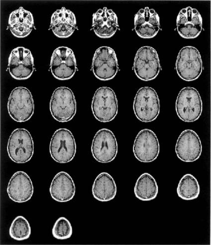
FIGURE 10.5 Montage display of 27 frames of magnetic resonance images of the brain plotted in Example 10.4. These multiframe images were obtained from MATLAB’s mri.tif file in the images section of the Image Processing Toolbox. Used with permission from MATLAB, Inc. Copyright 1993–2003, The Math Works, Inc. Reprinted with permission.

Copyright 2004 by Marcel Dekker, Inc. All Rights Reserved.

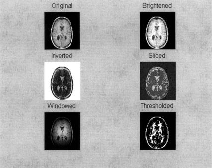
FIGURE 10.6 Figure showing various signal processing operations on frame 17 of the MRI images shown in Figure 10.5. Original from the MATLAB Image Processing Toolbox. Copyright 1993–2003, The Math Works, Inc. Reprinted with permission.

% Display original and all modifications on the same figure

%

%Initialize an array to hold 27 frames of mri.tif

%Since this image is stored in tif format, it could be in either

%unit8 or uint16.

%In fact, the specific input format will not matter, since it

%will be converted to double format in this program.

Copyright 2004 by Marcel Dekker, Inc. All Rights Reserved.

[mri(:,:,:,frame), map ] = imread(’mri.tif’, frame); end

montage(mri, map);

%

frame_select = input(’Select frame for processing: ’);

%Now check to see if image is Indexed (in fact ’whos’ shows it

%is).

if isempty(map) == 0

I = ind2gray(I,map);

end

I1 = im2double(I);

%

I_bright = immultiply(I1,1.2); I_invert = imcomplement(I1); x_slice = grayslice(I1,N_slice);

subplot(3,2,2);

imshow(I_bright), title(’Brightened’); subplot(3,2,3);

Copyright 2004 by Marcel Dekker, Inc. All Rights Reserved.

Since the image file might be indexed (in fact it is), the imread function includes map as an output. If the image is not indexed, then map will be empty. Note that imread reads only one frame at a time, the frame specified as the second argument of imread. To read in all 27 frames, it is necessary to use a loop. All frames are then displayed in one figure (Figure 10.5) using the montage function. The user is asked to select one frame for further processing. Since montage can display any input class and format, it is not necessary to determine these data characteristics at this time.

After a particular frame is selected, the program checks if the map variable is empty (function isempty). If it is not (as is the case for these data), then the image data is converted to grayscale using function ind2gray which produces an intensity image in double format. If the image is not Indexed, the image variable is converted to double format. The program then performs the various signal processing operations. Brightening is done by multiplying the image by a constant greater that 1.0, in this case 1.2, Figure 10.6. Inversion is done using imcomplement, and the image is sliced into N_slice (5) levels using grayslice. Since grayslice produces an indexed image, it also generates a map variable. However, this grayscale map is not used, rather an alternative map is substituted to produce a color image, with the color being used to enhance certain features of the image.* The Hanning window is applied to the image in both the horizontal and vertical direction Figure 10.6. Since the image, I1, is in double format, the multiplication can be carried out directly on the image array; however, the resultant array, I_window, has to be rescaled using mat2gray to insure it has the correct range for imshow. Recall that if called without any arguments; mat2gray scales the array to take up the full intensity range (i.e., 0 to 1). To place all the images in the same figure, subplot is used just as with other graphs, Figure 10.6. One potential problem with this approach is that Indexed data may plot incorrectly due to limited display memory allocated to

*More accurately, the image should be termed a pseudocolor image since the original data was grayscale. Unfortunately the image printed in this text is in grayscale; however the example can be rerun by the reader to obtain the actual color image.

Copyright 2004 by Marcel Dekker, Inc. All Rights Reserved.