Biosignal and Biomedical Image Processing MATLAB based Applications - John L. Semmlow

Two important properties of a random variable are its mean, or average value, and its variance, the term σ2 in Eq. (1). The arithmetic quantities of mean and variance are frequently used in signal processing algorithms, and their computation is well-suited to discrete data.

The mean value of a discrete array of N samples is evaluated as:

N

x¯ = 1 ∑ xk (2)

N k=1

Note that the summation in Eq. (2) is made between 1 and N as opposed to 0 and N − 1. This protocol will commonly be used throughout the text to be compatible with MATLAB notation where the first element in an array has an index of 1, not 0.

Frequently, the mean will be subtracted from the data sample to provide data with zero mean value. This operation is particularly easy in MATLAB as described in the next section. The sample variance, σ2, is calculated as shown in Eq. (3) below, and the standard deviation, σ, is just the square root of the variance.

Normalizing the standard deviation or variance by 1/N − 1 as in Eq. (3) produces the best estimate of the variance, if x is a sample from a Gaussian distribution. Alternatively, normalizing the variance by 1/N produces the second moment of the data around x. Note that this is the equivalent of the RMS value of the data if the data have zero as the mean.

When multiple measurements are made, multiple random variables can be generated. If these variables are combined or added together, the means add so that the resultant random variable is simply the mean, or average, of the individual means. The same is true for the variance—the variances add and the average variance is the mean of the individual variances:

N

σ 2 = 1 ∑ σ 2k (4)

N k=1

However, the standard deviation is the square root of the variance and the standard deviations add as the √N times the average standard deviation [Eq. (5)]. Accordingly, the mean standard deviation is the average of the individual standard deviations divided by √N [Eq. (6)].

From Eq. (4):

Copyright 2004 by Marcel Dekker, Inc. All Rights Reserved.

In other words, averaging noise from different sensors, or multiple observations from the same source, will reduce the standard deviation of the noise by the square root of the number of averages.

In addition to a mean and standard deviation, noise also has a spectral characteristic—that is, its energy distribution may vary with frequency. As shown below, the frequency characteristics of the noise are related to how well one instantaneous value of noise correlates with the adjacent instantaneous values: for digitized data how much one data point is correlated with its neighbors. If the noise has so much randomness that each point is independent of its neighbors, then it has a flat spectral characteristic and vice versa. Such noise is called white noise since it, like white light, contains equal energy at all frequencies (see Figure 1.5). The section on Noise Sources in Chapter 1 mentioned that most electronic sources produce noise that is essentially white up to many megahertz. When white noise is filtered, it becomes bandlimited and is referred to as colored noise since, like colored light, it only contains energy at certain frequencies. Colored noise shows some correlation between adjacent points, and this correlation becomes stronger as the bandwidth decreases and the noise becomes more monochromatic. The relationship between bandwidth and correlation of adjacent points is explored in the section on autocorrelation.

ENSEMBLE AVERAGING

Eq. (6) indicates that averaging can be a simple, yet powerful signal processing technique for reducing noise when multiple observations of the signal are possible. Such multiple observations could come from multiple sensors, but in many biomedical applications, the multiple observations come from repeated responses to the same stimulus. In ensemble averaging, a group, or ensemble, of time responses are averaged together on a point-by-point basis; that is, an average signal is constructed by taking the average, for each point in time, over all signals in the ensemble (Figure 2.2). A classic biomedical engineering example of the application of ensemble averaging is the visual evoked response (VER) in which a visual stimulus produces a small neural signal embedded in the EEG. Usually this signal cannot be detected in the EEG signal, but by averaging hundreds of observations of the EEG, time-locked to the visual stimulus, the visually evoked signal emerges.

There are two essential requirements for the application of ensemble averaging for noise reduction: the ability to obtain multiple observations, and a reference signal closely time-linked to the response. The reference signal shows how the multiple observations are to be aligned for averaging. Usually a time

Copyright 2004 by Marcel Dekker, Inc. All Rights Reserved.

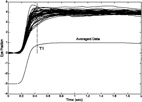
FIGURE 2.2 Upper traces: An ensemble of individual (vergence) eye movement responses to a step change in stimulus. Lower trace: The ensemble average, displaced downward for clarity. The ensemble average is constructed by averaging the individual responses at each point in time. Hence, the value of the average response at time T1 (vertical line) is the average of the individual responses at that time.

signal linked to the stimulus is used. An example of ensemble averaging is shown in Figure 2.2, and the code used to produce this figure is presented in the following MATLAB implementation section.

MATLAB IMPLEMENTATION

In MATLAB the mean, variance, and standard deviations are implemented as shown in the three code lines below.

Copyright 2004 by Marcel Dekker, Inc. All Rights Reserved.

If x is an array (also termed a vector for reasons given later) the output of these function calls is a scalar representing the mean, variance, or standard deviation. If x is a matrix then the output is a row vector resulting from applying the appropriate calculation (mean, variance, or standard deviation) to each column of the matrix.

Example 2.1 below shows the implementation of ensemble averaging that produced the data in Figure 2.2. The program first loads the eye movement data (load verg1), then plots the ensemble. The ensemble average is determined using the MATLAB mean routine. Note that the data matrix, data_out, must be in the correct orientation (the responses must be in rows) for routine mean. If that were not the case (as in Problem 1 at the end of this chapter), the matrix transposition operation should be performed*. The ensemble average, avg, is then plotted displaced by 3 degrees to provide a clear view. Otherwise it would overlay the data.

Example 2.1 Compute and display the Ensemble average of an ensemble of vergence eye movement responses to a step change in stimulus. These responses are stored in MATLAB file verg1.mat.

%Example 2.1 and Figure 2.2 Load eye movement data, plot

%the data then generate and plot the ensemble average.

close all; clear all;

%

%Plot ensemble data superimposed plot(t,data_out,‘k’);

hold on;

%Construct and plot the ensemble average

*In MATLAB, matrix or vector transposition is indicated by an apostrophe following the variable. For example if x is a row vector, x′ is a column vector and visa versa. If X is a matrix, X′ is that matrix with rows and columns switched.

Copyright 2004 by Marcel Dekker, Inc. All Rights Reserved.

DATA FUNCTIONS AND TRANSFORMS

To mathematicians, the term function can take on a wide range of meanings. In signal processing, most functions fall into two categories: waveforms, images, or other data; and entities that operate on waveforms, images, or other data (Hubbard, 1998). The latter group can be further divided into functions that modify the data, and functions used to analyze or probe the data. For example, the basic filters described in Chapter 4 use functions (the filter coefficients) that modify the spectral content of a waveform while the Fourier Transform detailed in Chapter 3 uses functions (harmonically related sinusoids) to analyze the spectral content of a waveform. Functions that modify data are also termed operations or transformations.

Since most signal processing operations are implemented using digital electronics, functions are represented in discrete form as a sequence of numbers:

Discrete data functions (waveforms or images) are usually obtained through analog-to-digital conversion or other data input, while analysis or modifying functions are generated within the computer or are part of the computer program. (The consequences of converting a continuous time function into a discrete representation are described in the section below on sampling theory.)

In some applications, it is advantageous to think of a function (of whatever type) not just as a sequence, or array, of numbers, but as a vector. In this conceptualization, x(n) is a single vector defined by a single point, the endpoint of the vector, in N-dimensional space, Figure 2.3. This somewhat curious and highly mathematical concept has the advantage of unifying some signal processing operations and fits well with matrix methods. It is difficult for most people to imagine higher-dimensional spaces and even harder to present them graphically, so operations and functions in higher-dimensional space are usually described in 2 or 3 dimensions, and the extension to higher dimensional space is left to the imagination of the reader. (This task can sometimes be difficult for nonmathematicians: try and imagine a data sequence of even a 32-point array represented as a single vector in 32-dimensional space!)

A transform can be thought of as a re-mapping of the original data into a function that provides more information than the original.* The Fourier Transform described in Chapter 3 is a classic example as it converts the original time

*Some definitions would be more restrictive and require that a transform be bilateral; that is, it must be possible to recover the original signal from the transformed data. We will use the looser definition and reserve the term bilateral transform to describe reversible transformations.

Copyright 2004 by Marcel Dekker, Inc. All Rights Reserved.

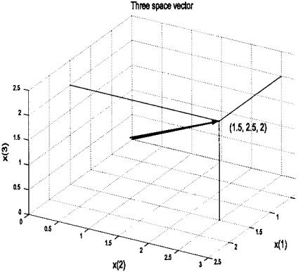
FIGURE 2.3 The data sequence x(n) = [1.5,2.5,2] represented as a vector in three-dimensional space.

data into frequency information which often provides greater insight into the nature and/or origin of the signal. Many of the transforms described in this text are achieved by comparing the signal of interest with some sort of probing function. This comparison takes the form of a correlation (produced by multiplication) that is averaged (or integrated) over the duration of the waveform, or some portion of the waveform:

where x(t) is the waveform being analyzed, fm(t) is the probing function and m is some variable of the probing function, often specifying a particular member in a family of similar functions. For example, in the Fourier Transform fm(t) is a family of harmonically related sinusoids and m specifies the frequency of an

Copyright 2004 by Marcel Dekker, Inc. All Rights Reserved.

individual sinusoid in that family (e.g., sin(mft)). A family of probing functions is also termed a basis. For discrete functions, a probing function consists of a sequence of values, or vector, and the integral becomes summation over a finite range:

n=1

where x(n) is the discrete waveform and fm(n) is a discrete version of the family of probing functions. This equation assumes the probe and waveform functions are the same length. Other possibilities are explored below.

When either x(t) or fm(t) are of infinite length, they must be truncated in some fashion to fit within the confines of limited memory storage. In addition, if the length of the probing function, fm(n), is shorter than the waveform, x(n), then x(n) must be shortened in some way. The length of either function can be shortened by simple truncation or by multiplying the function by yet another function that has zero value beyond the desired length. A function used to shorten another function is termed a window function, and its action is shown in Figure 2.4. Note that simple truncation can be viewed as multiplying the function by a rectangular window, a function whose value is one for the portion of the function that is retained, and zero elsewhere. The consequences of this artificial shortening will depend on the specific window function used. Consequences of data windowing are discussed in Chapter 3 under the heading Window Functions. If a window function is used, Eq. (8) becomes:

n=1

where W(n) is the window function. In the Fourier Transform, the length of W(n) is usually set to be the same as the available length of the waveform, x(n), but in other applications it can be shorter than the waveform. If W(n) is a rectangular function, then W(n) =1 over the length of the summation (1 ≤ n ≤ N), and it is usually omitted from the equation. The rectangular window is implemented implicitly by the summation limits.

If the probing function is of finite length (in mathematical terms such a function is said to have finite support) and this length is shorter than the waveform, then it might be appropriate to translate or slide it over the signal and perform the comparison (correlation, or multiplication) at various relative positions between the waveform and probing function. In the example shown in Figure 2.5, a single probing function is shown (representing a single family member), and a single output function is produced. In general, the output would be a family of functions, or a two-variable function, where one variable corresponds to the relative position between the two functions and the other to the

Copyright 2004 by Marcel Dekker, Inc. All Rights Reserved.

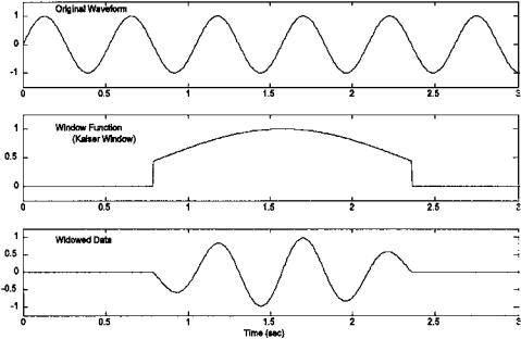
FIGURE 2.4 A waveform (upper plot) is multiplied by a window function (middle plot) to create a truncated version (lower plot) of the original waveform. The window function is shown in the middle plot. This particular window function is called the Kaiser Window, one of many popular window functions.

specific family member. This sliding comparison is similar to convolution described in the next section, and is given in discrete form by the equation:

n=1

where the variable k indicates the relative position between the two functions and m is the family member as in the above equations. This approach will be used in the filters described in Chapter 4 and in the Continuous Wavelet Transform described in Chapter 7. A variation of this approach can be used for long—or even infinite—probing functions, provided the probing function itself is shortened by windowing to a length that is less than the waveform. Then the shortened probing function can be translated across the waveform in the same manner as a probing function that is naturally short. The equation for this condition becomes:

Copyright 2004 by Marcel Dekker, Inc. All Rights Reserved.

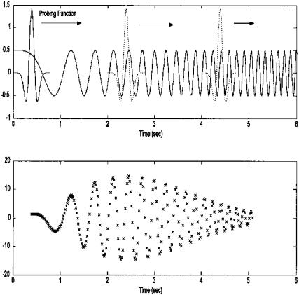
FIGURE 2.5 The probing function slides over the waveform of interest (upper panel) and at each position generates the summed, or averaged, product of the two functions (lower panel), as in Eq. (10). In this example, the probing function is one member of the “Mexican Hat” family (see Chapter 7) and the waveform is a sinusoid that increases its frequency linearly over time (known as a chirp.) The summed product (lower panel), also known as the scalar product, shows the relative correlation between the waveform and the probing function as it slides across the waveform. Note that this relative correlation varies sinusoidally as the phase between the two functions varies, but reaches a maximum around 2.5 sec, the time when the waveform is most like the probing function.

Copyright 2004 by Marcel Dekker, Inc. All Rights Reserved.

n=1

where fm(n) is a longer function that is shortened by the sliding window function, (W(n − k), and the variables m and k have the same meaning as in Eq. (10). This is the approach taken in the Short-Term Fourier Transform described in Chapter 6.

All of the discrete equations above, Eqs. (7) to (11), have one thing in common: they all feature the multiplication of two (or sometimes three) functions and the summation of the product over some finite interval. Returning to the vector conceptualization for data sequences mentioned above (see Figure 2.3), this multiplication and summation is the same as scalar product of the two vectors.*

Note that the scalar product results in a single number (i.e., a scalar), not a vector. The scalar product can also be defined in terms of the magnitude of the two vectors and the angle between them:

where θ is the angle between the two vectors. If the two vectors are perpendicular to one another, i.e., they are orthogonal, then θ = 90°, and their salar product will be zero. Eq. (13) demonstrates that the scalar product between waveform and probe function is mathematically the same as a projection of the waveform vector onto the probing function vector (after normalizing by probe vector length). When the probing function consists of a family of functions, then the scalar product operations in Eqs. (7)–(11) can be thought of as projecting the waveform vector onto vectors representing the various family members. In this vector-based conceptualization, the probing function family, or basis, can be thought of as the axes of a coordinate system. This is the motivation behind the development of probing functions that have family members that are orthogonal,

*The scalar product is also termed the inner product, the standard inner product, or the dot product.

Copyright 2004 by Marcel Dekker, Inc. All Rights Reserved.