Biosignal and Biomedical Image Processing MATLAB based Applications - John L. Semmlow

replaced by the filter coefficients, b(n). Hence, FIR filters can be implemented using either convolution or MATLAB’s filter routine. Eq. (8) indicates that the filter coefficients (or weights) of an FIR filter are the same as the impulse response of the filter. Since the frequency response of a process having an impulse response h(n) is simply the Fourier transform of h(n), the frequency response of an FIR filter having coefficients b(n) is just the Fourier transform of b(n):

n=0

Eq. (9) is a special case of Eq. (5) when the denominator equals one. If b(n) generally consists of a small number of elements, this equation can sometimes be determined manually as well as by computer.

The inverse operation, going from a desired frequency response to the coefficient function, b(n), is known as filter design. Since the frequency response is the Fourier transform of the filter coefficients, the coefficients can be found from the inverse Fourier transform of the desired frequency response. This design strategy is illustrated below in the design of a FIR lowpass filter based on the spectrum of an ideal filter. This filter is referred to as a rectangular window filter* since its spectrum is ideally a rectangular window.

FIR Filter Design

The ideal lowpass filter was first introduced in Chapter 1 as a rectangular window in the frequency domain (Figure 1.7). The inverse Fourier transform of a rectangular window function is given in Eq. (25) in Chapter 2 and repeated here with a minor variable change:

= sin[2πfcTs(n − L/2)]

b(n) (10) π(n − L/2)

where fc is the cutoff frequency; Ts is the sample interval in seconds; and L is the length of the filter. The argument, n − L/2, is used to make the coefficient function symmetrical giving the filter linear phase characteristics. Linear phase characteristics are a desirable feature not easily attainable with IIR filters. The coefficient function, b(n), produced by Eq. (10), is shown for two values of fc in Figure 4.4. Again, this function is the same as the impulse response. Unfortu-

*This filter is sometimes called a window filter, but the term rectangular window filter will be used in this text so as not to confuse the filter with a window function as described in the last chapter. This can be particularly confusing since, as we show later, rectangular window filters also use window functions!

Copyright 2004 by Marcel Dekker, Inc. All Rights Reserved.

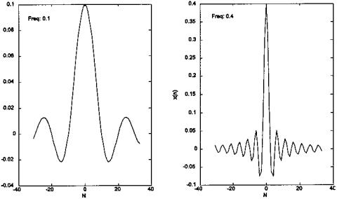
FIGURE 4.4 Symmetrical weighting function of a rectangular filter (Eq. (10) truncated at 64 coefficients. The cutoff frequencies are given relative to the sampling frequency, fs, as is often done in discussing digital filter frequencies. Left: Lowpass filter with a cutoff frequency of 0.1fs /2 Hz. Right: Lowpass cutoff frequency of 0.4fs /2 Hz.

nately this coefficient function must be infinitely long to produce the filter characteristics of an ideal filter; truncating it will result in a lowpass filter that is less than ideal. Figure 4.5 shows the frequency response, obtained by taking the Fourier transform of the coefficients for two different lengths. This filter also shows a couple of artifacts associated with finite length: an oscillation in the frequency curve which increases in frequency when the coefficient function is longer, and a peak in the passband which becomes narrower and higher when the coefficient function is lengthened.

Since the artifacts seen in Figure 4.5 are due to truncation of an (ideally) infinite function, we might expect that some of the window functions described in Chapter 3 would help. In discussing window frequency characteristics in Chapter 3, we noted that it is desirable to have a narrow mainlobe and rapidly diminishing sidelobes, and that the various window functions were designed to make different compromises between these two features. When applied to an FIR weight function, the width of the mainlobe will influence the sharpness of the transition band, and the sidelobe energy will influence the oscillations seen

Copyright 2004 by Marcel Dekker, Inc. All Rights Reserved.

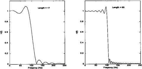
FIGURE 4.5 Freuquency characteristics of an FIR filter based in a weighting function derived from Eq. (10). The weighting functions were abruptly truncated at 17 and 65 coefficients. The artifacts associated with this truncation are clearly seen. The lowpass cutoff frequency is 100 Hz.

in Figure 4.5. Figure 4.6 shows the frequency characteristics that are produced by the same coefficient function used in Figure 4.4 except that a Hamming window has been applied to the filter weights. The artifacts are considerably diminished by the Hamming window: the overshoot in the passband has disappeared and the oscillations are barely visible in the plot. As with the unwindowed filter, there is a significant improvement in the sharpness of the transition band for the filter when more coefficients are used.

The FIR filter coefficients for highpass, bandpass, and bandstop filters can be derived in the same manner from equations generated by applying an inverse FT to rectangular structures having the appropriate associated shape. These equations have the same general form as Eq. (10) except they include additional terms:

Copyright 2004 by Marcel Dekker, Inc. All Rights Reserved.

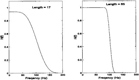
FIGURE 4.6 Frequency characteristics produced by an FIR filter identical to the one used in Figure 4.5 except a Hamming function has been applied to the filter coefficients. (See Example 1 for the MATLAB code.)

An FIR bandpass filter designed using Eq. (12) is shown in Figure 4.7 for two different truncation lengths. Implementation of other FIR filter types is a part of the problem set at the end of this chapter. A variety of FIR filters exist that use strategies other than the rectangular window to construct the filter coefficients, and some of these are explored in the section on MATLAB implementation. One FIR filter of particular interest is the filter used to construct the derivative of a waveform since the derivative is often of interest in the analysis of biosignals. The next section explores a popular filter for this operation.

Derivative Operation: The Two-Point Central

Difference Algorithm

The derivative is a common operation in signal processing and is particularly useful in analyzing certain physiological signals. Digital differentiation is de-

Copyright 2004 by Marcel Dekker, Inc. All Rights Reserved.

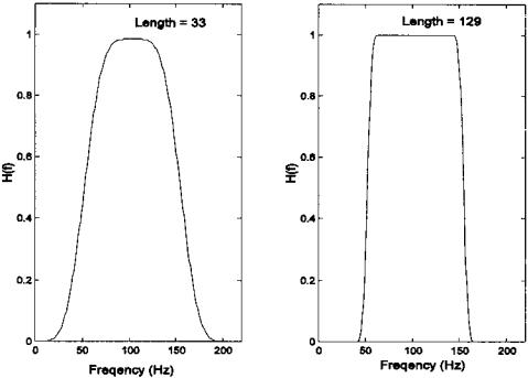
FIGURE 4.7 Frequency characteristics of an FIR Bandpass filter with a coefficient function described by Eq. (12) in conjuction with the Blackman window function. The low and high cutoff frequencies were 50 and 150 Hz. The filter function was truncated at 33 and 129 coefficients. These figures were generated with code similar to that in Example 4.2 below, except modified according to Eq. (12)

fined as ∆x/∆t and can be implemented by taking the difference between two adjacent points, scaling by 1/Ts, and repeating this operation along the entire waveform. In the context of the FIR filters described above, this is equivalent to a two coefficient filter, [−1, +1]/Ts, and this is the approach taken by MATLAB’s derv routine. The frequency characteristic of the derivative operation is a linear increase with frequency, Figure 4.8 (dashed line) so there is considerable gain at the higher frequencies. Since the higher frequencies frequently contain a greater percentage of noise, this operation tends to produce a noisy derivative curve. Figure 4.9A shows a noisy physiological motor response (vergence eye movements) and the derivative obtained using the derv function. Figure 4.9B shows the same response and derivative when the derivative was calculated using the two-point central difference algorithm. This algorithm acts

Copyright 2004 by Marcel Dekker, Inc. All Rights Reserved.

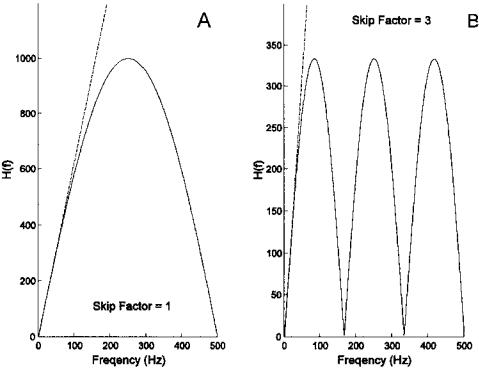
FIGURE 4.8 The frequency response of the two-point central difference algorithm using two different values for the skip factor: (A) L = 1; (B) L = 4. The sample time was 1 msec.

as a differentiator for the lower frequencies and as an integrator (or lowpass filter) for higher frequencies.

The two-point central difference algorithm uses two coefficients of equal but opposite value spaced L points apart, as defined by the input–output equation:

where L is the skip factor that influences the effective bandwidth as described below, and Ts is the sample interval. The filter coefficients for the two-point central difference algorithm would be:

Copyright 2004 by Marcel Dekker, Inc. All Rights Reserved.

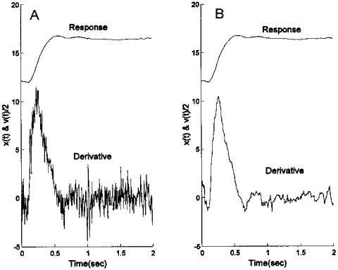
FIGURE 4.9 A physiological motor response to a step input is shown in the upper trace and its derivative is shown in the lower trace. (A) The derivative was calculated by taking the difference in adjacent points and scaling by the sample frequency. (B) The derivative was computed using the two-point central difference algorithm with a skip factor of 4. Derivative functions were scaled by 1/2 and responses were offset to improve viewing.

The frequency response of this filter algorithm can be determined by taking the Fourier transform of the filter coefficient function. Since this function contains only two coefficients, the Fourier transform can be done either analyti-

Copyright 2004 by Marcel Dekker, Inc. All Rights Reserved.

cally or using MATLAB’s fft routine. Both methods are presented in the example below.

Example 4.2 Determine the frequency response of the two-point central difference algorithm.

Analytical: Since the coefficient function is nonzero only for n = ± L, the Fourier transform, after adjusting the summation limits for a symmetrical coefficient function with positive and negative n, becomes:

where L is the skip factor and N is the number of samples in the waveform. To put Eq. (16) in terms of frequency, note that f = m/(NTs); hence, m = f NTs. Substituting:

Eq. (17) shows that *X(k)* is a sine function that goes to zero at f = 1/(LTs) or fs/L. Figure 4.8 shows the frequency characteristics of the two-point central difference algorithm for two different skip factors, and the MATLAB code used to calculate and plot the frequency plot is shown in Example 4.2. A true derivative would have a linear change with frequency (specifically, a line with a slope of 2πf ) as shown by the dashed lines in Figure 4.8. The two-point central difference curves approximate a true derivative for the lower frequencies, but has the characteristic of a lowpass filter for higher frequencies. Increasing the skip factor, L, has the effect of lowering the frequency range over which the filter acts like a derivative operator as well as the lowpass filter range. Note that for skip factors >1, the response curve repeats above f = 1/(LTs). Usually the assumption is made that the signal does not contain frequencies in this range. If this is not true, then these higher frequencies could be altered by the frequency characteristics of this filter above 1/(LTs).

MATLAB Implementation

Since the FIR coefficient function is the same as the impulse response of the filter process, design and application of these filters can be achieved using only FFT and convolution. However, the MATLAB Signal Processing Toolbox has a number of useful FIR filter design routines that greatly facilitate the design of FIR filters, particularly if the desired frequency response is complicated. The

Copyright 2004 by Marcel Dekker, Inc. All Rights Reserved.

following two examples show the application use of FIR filters using only convolution and the FFT, followed by a discussion and examples of FIR filter design using MATLAB’s Signal Processing Toolbox.

Example 4.2 Generate the coefficient function for the two-point central difference derivative algorithm and plot the frequency response. This program was used to generate the plots in Figure 4.8.

%Example 4.2 and Figure 4.8

%Program to determine the frequency response

%of the two point central difference algorithm for

%differentiation

axis([0 500 0 max(H) .2*max(H)]); text(100,max(H),[’Skip Factor = ’,Num2str(L)]); xlabel(’Frequency (Hz)’); ylabel(’H(f)’);

Note that the second to fourth lines of the for loop are used to build the filter coefficients, b(n), for the given skip factor, L. The next line takes the absolute value of the Fourier transform of this function. The coefficient function is zero-padded out to 1000 points, both to improve the appearance of the result-

Copyright 2004 by Marcel Dekker, Inc. All Rights Reserved.

ing frequency response curve and to simulate the application of the filter to a 1000 point data array sampled at 1 kHz.

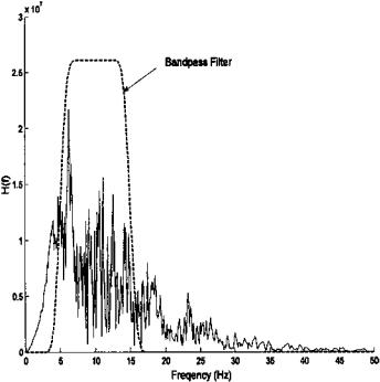
Example 4.3 Develop and apply an FIR bandpass filter to physiological data. This example presents the construction and application of a narrowband filter such as shown in Figure 4.10 (right side) using convolution. The data are from a segment of an EEG signal in the PhysioNet data bank (http://www. physionet.org). A spectrum analysis is first performed on both the data and the filter to show the range of the filter’s operation with respect to the frequency spectrum of the data. The standard FFT is used to analyze the data without windowing or averaging. As shown in Figure 4.10, the bandpass filter transmits most of the signal’s energy, attenuating only a portion of the low frequency and

FIGURE 4.10 Frequency spectrum of EEG data shown in Figure 4.11 obtained using the FFT. Also shown is the frequency response of an FIR bandpass filter constructed using Eq. (12). The MATLAB code that generated this figure is presented in Example 4.3.

Copyright 2004 by Marcel Dekker, Inc. All Rights Reserved.