Biosignal and Biomedical Image Processing MATLAB based Applications - John L. Semmlow

since the matrix has the Toeplitz structure, matrix inversion can also be done using a faster algorithm known as the Levinson-Durbin recursion.

The MATLAB toeplitz function is useful in setting up the correlation matrix. The function call is:

Rxx = toeplitz(rxx);

where rxx is the input row vector. This constructs a symmetrical matrix from a single row vector and can be used to generate the correlation matrix in Eq. (6) from the autocorrelation function rxx. (The function can also create an asymmetrical Toeplitz matrix if two input arguments are given.)

In order for the matrix to be inverted, it must be nonsingular; that is, the rows and columns must be independent. Because of the structure of the correlation matrix in Eq. (6) (termed positive- definite), it cannot be singular. However, it can be near singular: some rows or columns may be only slightly independent. Such an ill-conditioned matrix will lead to large errors when it is inverted. The MATLAB ‘\’ matrix inversion operator provides an error message if the matrix is not well-conditioned, but this can be more effectively evaluated using the MATLAB cond function:

c = cond(X)

where X is the matrix under test and c is the ratio of the largest to smallest singular values. A very well-conditioned matrix would have singular values in the same general range, so the output variable, c, would be close to one. Very large values of c indicate an ill-conditioned matrix. Values greater than 104 have been suggested by Sterns and David (1996) as too large to produce reliable results in the Wiener-Hopf equation. When this occurs, the condition of the matrix can usually be improved by reducing its dimension, that is, reducing the range, L, of the autocorrelation function in Eq (6). This will also reduce the number of filter coefficients in the solution.

Example 8.1 Given a sinusoidal signal in noise (SNR = -8 db), design an optimal filter using the Wiener-Hopf equation. Assume that you have a copy of the actual signal available, in other words, a version of the signal without the added noise. In general, this would not be the case: if you had the desired signal, you would not need the filter! In practical situations you would have to estimate the desired signal or the crosscorrelation between the estimated and desired signals.

Solution The program below uses the routine wiener_hopf (also shown below) to determine the optimal filter coefficients. These are then applied to the noisy waveform using the filter routine introduced in Chapter 4 although correlation could also have been used.

Copyright 2004 by Marcel Dekker, Inc. All Rights Reserved.

%Example 8.1 and Figure 8.3 Wiener Filter Theory

%Use an adaptive filter to eliminate broadband noise from a

%narrowband signal

%Implemented using Wiener-Hopf equations

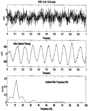
FIGURE 8.3 Application of the Wiener-Hopf equation to produce an optimal FIR filter to filter broadband noise (SNR = -8 db) from a single sinusoid (10 Hz.) The frequency characteristics (bottom plot) show that the filter coefficients were adjusted to approximate a bandpass filter with a small bandwidth and a peak at 10 Hz.

Copyright 2004 by Marcel Dekker, Inc. All Rights Reserved.

%

%Generate signal and noise data: 10 Hz sin in 8 db noise (SNR =

%-8 db)

..........labels, table, axis.........

%

% Determine the optimal FIR filter coefficients and apply

..........labels, table, axis.........

The function Wiener_hopf solves the Wiener-Hopf equations:

function b = wiener_hopf(x,y,maxlags)

% Function to compute LMS algol using Wiener-Hopf equations

%

rxx = xcorr(x,maxlags,’coeff’);

rxx = rxx(maxlags 1:end)’;

rxy = xcorr(x,y,maxlags);

rxy = rxy(maxlags 1:end)’;

%

rxx_matrix = toeplitz(rxx);

Copyright 2004 by Marcel Dekker, Inc. All Rights Reserved.

Example 8.1 generates Figure 8.3 above. Note that the optimal filter approach, when applied to a single sinusoid buried in noise, produces a bandpass filter with a peak at the sinusoidal frequency. An equivalent—or even more effective—filter could have been designed using the tools presented in Chapter 4. Indeed, such a statement could also be made about any of the adaptive filters described below. However, this requires precise a priori knowledge of the signal and noise frequency characteristics, which may not be available. Moreover, a fixed filter will not be able to optimally filter signal and noise that changes over time.

Example 8.2 Apply the LMS algorithm to a systems identification task. The “unknown” system will be an all-zero linear process with a digital transfer function of:

H(z) = 0.5 + 0.75z−1 + 1.2z−2

Confirm the match by plotting the magnitude of the transfer function for both the unknown and matching systems. Since this approach uses an FIR filter as the matching system, which is also an all-zero process, the match should be quite good. In Problem 2, this approach is repeated, but for an unknown system that has both poles and zeros. In this case, the FIR (all-zero) filter will need many more coefficients than the unknown pole-zero process to produce a reasonable match.

Solution The program below inputs random noise into the unknown process using convolution and into the matching filter. Since the FIR matching filter cannot easily accommodate for a pure time delay, care must be taken to compensate for possible time shift due to the convolution operation. The matching filter coefficients are adjusted using the Wiener-Hopf equation described previously. Frequency characteristics of both unknown and matching system are determined by applying the FFT to the coefficients of both processes and the resultant spectra are plotted.

%Example 8.2 and Figure 8.4 Adaptive Filters System

%Identification

%

%Uses optimal filtering implemented with the Wiener-Hopf

%algorithm to identify an unknown system

%

% Initialize parameters

Copyright 2004 by Marcel Dekker, Inc. All Rights Reserved.

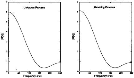
FIGURE 8.4 Frequency characteristics of an “unknown” process having coefficients of 0.5, 0.75, and 1.2 (an all-zero process). The matching process uses system identification implemented with the Wiener-Hopf adaptive filtering approach. This matching process generates a linear system with a similar spectrum to the unknown process. Since the unknown process is also an all-zero system, the transfer function coefficients also match.

%

% Generate unknown system and noise input

% Calculate frequency characteristics using the FFT ps_match = (abs(fft(b,N))).v2;

ps_unknown = (abs(fft(b_unknown,N))).v2;

Copyright 2004 by Marcel Dekker, Inc. All Rights Reserved.

%

%Plot frequency characteristics of unknown and identified

%process

plot(f(1:N/2),ps_unknown(1:N/2),’k’);

..........labels, table, axis.........

subplot(1,2,2);

% Plot matching system freq. char.

plot(f(1:N/2),ps_match(1:N/2),’k’);

..........labels, table, axis.........

The output plots from this example are shown in Figure 8.4. Note the close match in spectral characteristics between the “unknown” process and the matching output produced by the Wiener-Hopf algorithm. The transfer functions also closely match as seen by the similarity in impulse response coefficients:

ADAPTIVE SIGNAL PROCESSING

The area of adaptive signal processing is relatively new yet already has a rich history. As with optimal filtering, only a brief example of the usefulness and broad applicability of adaptive filtering can be covered here. The FIR and IIR filters described in Chapter 4 were based on an a priori design criteria and were fixed throughout their application. Although the Wiener filter described above does not require prior knowledge of the input signal (only the desired outcome), it too is fixed for a given application. As with classical spectral analysis methods, these filters cannot respond to changes that might occur during the course of the signal. Adaptive filters have the capability of modifying their properties based on selected features of signal being analyzed.

A typical adaptive filter paradigm is shown in Figure 8.5. In this case, the filter coefficients are modified by a feedback process designed to make the filter’s output, y(n), as close to some desired response, d(n), as possible, by reducing the error, e(n), to a minimum. As with optimal filtering, the nature of the desired response will depend on the specific problem involved and its formulation may be the most difficult part of the adaptive system specification (Stearns and David, 1996).

The inherent stability of FIR filters makes them attractive in adaptive applications as well as in optimal filtering (Ingle and Proakis, 2000). Accordingly, the adaptive filter, H(z), can again be represented by a set of FIR filter coefficients,

Copyright 2004 by Marcel Dekker, Inc. All Rights Reserved.

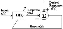
FIGURE 8.5 Elements of a typical adaptive filter.

b(k). The FIR filter equation (i.e., convolution) is repeated here, but the filter coefficients are indicated as bn(k) to indicate that they vary with time (i.e., n).

k=1

The adaptive filter operates by modifying the filter coefficients, bn(k), based on some signal property. The general adaptive filter problem has similarities to the Wiener filter theory problem discussed above in that an error is minimized, usually between the input and some desired response. As with optimal filtering, it is the squared error that is minimized, and, again, it is necessary to somehow construct a desired signal. In the Wiener approach, the analysis is applied to the entire waveform and the resultant optimal filter coefficients were similarly applied to the entire waveform (a so-called block approach). In adaptive filtering, the filter coefficients are adjusted and applied in an ongoing basis.

While the Wiener-Hopf equations (Eqs. (6) and (7)) can be, and have been, adapted for use in an adaptive environment, a simpler and more popular approach is based on gradient optimization. This approach is usually called the LMS recursive algorithm. As in Wiener filter theory, this algorithm also determines the optimal filter coefficients, and it is also based on minimizing the squared error, but it does not require computation of the correlation functions, rxx and rxy. Instead the LMS algorithm uses a recursive gradient method known as the steepest-descent method for finding the filter coefficients that produce the minimum sum of squared error.

Examination of Eq. (3) shows that the sum of squared errors is a quadratic function of the FIR filter coefficients, b(k); hence, this function will have a single minimum. The goal of the LMS algorithm is to adjust the coefficients so that the sum of squared error moves toward this minimum. The technique used by the LMS algorithm is to adjust the filter coefficients based on the method of steepest descent. In this approach, the filter coefficients are modified based on

Copyright 2004 by Marcel Dekker, Inc. All Rights Reserved.

an estimate of the negative gradient of the error function with respect to a given b(k). This estimate is given by the partial derivative of the squared error, ε, with respect to the coefficients, bn(k):

Since d(n) is independent of the coefficients, bn(k), its partial derivative with respect to bn(k) is zero. As y(n) is a function of the input times bn(k) (Eq. (8)), then its partial derivative with respect to bn(k) is just x(n-k), and Eq. (9) can be rewritten in terms of the instantaneous product of error and the input:

Initially, the filter coefficients are set arbitrarily to some b0(k), usually zero. With each new input sample a new error signal, e(n), can be computed (Figure 8.5). Based on this new error signal, the new gradient is determined (Eq. (10)), and the filter coefficients are updated:

where ∆ is a constant that controls the descent and, hence, the rate of convergence. This parameter must be chosen with some care. A large value of ∆ will lead to large modifications of the filter coefficients which will hasten convergence, but can also lead to instability and oscillations. Conversely, a small value will result in slow convergence of the filter coefficients to their optimal values. A common rule is to select the convergence parameter, ∆, such that it lies in the range:

10LPx

where L is the length of the FIR filter and Px is the power in the input signal. PX can be approximated by:

Note that for a waveform of zero mean, Px equals the variance of x. The LMS algorithm given in Eq. (11) can easily be implemented in MATLAB, as shown in the next section.

Adaptive filtering has a number of applications in biosignal processing. It can be used to suppress a narrowband noise source such as 60 Hz that is corrupting a broadband signal. It can also be used in the reverse situation, removing broadband noise from a narrowband signal, a process known as adaptive line

Copyright 2004 by Marcel Dekker, Inc. All Rights Reserved.

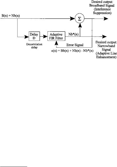
FIGURE 8.6 Configuration for Adaptive Line Enhancement (ALE) or Adaptive Interference Suppression. The Delay, D, decorrelates the narrowband component allowing the adaptive filter to use only this component. In ALE the narrowband component is the signal while in Interference suppression it is the noise.

enhancement (ALE).* It can also be used for some of the same applications as the Wiener filter such as system identification, inverse modeling, and, especially important in biosignal processing, adaptive noise cancellation. This last application requires a suitable reference source that is correlated with the noise, but not the signal. Many of these applications are explored in the next section on MATLAB implementation and/or in the problems.

The configuration for ALE and adaptive interference suppression is shown in Figure 8.6. When this configuration is used in adaptive interference suppression, the input consists of a broadband signal, Bb(n), in narrowband noise, Nb(n), such as 60 Hz. Since the noise is narrowband compared to the relatively broadband signal, the noise portion of sequential samples will remain correlated while the broadband signal components will be decorrelated after a few samples.† If the combined signal and noise is delayed by D samples, the broadband (signal) component of the delayed waveform will no longer be correlated with the broadband component in the original waveform. Hence, when the filter’s output is subtracted from the input waveform, only the narrowband component

*The adaptive line enhancer is so termed because the objective of this filter is to enhance a narrowband signal, one with a spectrum composed of a single “line.”

†Recall that the width of the autocorrelation function is a measure of the range of samples for which the samples are correlated, and this width is inversely related to the signal bandwidth. Hence, broadband signals remain correlated for only a few samples and vice versa.

Copyright 2004 by Marcel Dekker, Inc. All Rights Reserved.

can have an influence on the result. The adaptive filter will try to adjust its output to minimize this result, but since its output component, Nb*(n), only correlates with the narrowband component of the waveform, Nb(n), it is only the narrowband component that is minimized. In adaptive interference suppression, the narrowband component is the noise and this is the component that is minimized in the subtracted signal. The subtracted signal, now containing less noise, constitutes the output in adaptive interference suppression (upper output, Figure 8.6).

In adaptive line enhancement, the configuration is the same except the roles of signal and noise are reversed: the narrowband component is the signal and the broadband component is the noise. In this case, the output is taken from the filter output (Figure 8.6, lower output). Recall that this filter output is optimized for the narrowband component of the waveform.

As with the Wiener filter approach, a filter of equal or better performance could be constructed with the same number of filter coefficients using the traditional methods described in Chapter 4. However, the exact frequency or frequencies of the signal would have to be known in advance and these spectral features would have to be fixed throughout the signal, a situation that is often violated in biological signals. The ALE can be regarded as a self-tuning narrowband filter which will track changes in signal frequency. An application of ALE is provided in Example 8.3 and an example of adaptive interference suppression is given in the problems.

Adaptive Noise Cancellation

Adaptive noise cancellation can be thought of as an outgrowth of the interference suppression described above, except that a separate channel is used to supply the estimated noise or interference signal. One of the earliest applications of adaptive noise cancellation was to eliminate 60 Hz noise from an ECG signal (Widrow, 1964). It has also been used to improve measurements of the fetal ECG by reducing interference from the mother’s EEG. In this approach, a reference channel carries a signal that is correlated with the interference, but not with the signal of interest. The adaptive noise canceller consists of an adaptive filter that operates on the reference signal, N’(n), to produce an estimate of the interference, N(n) (Figure 8.7). This estimated noise is then subtracted from the signal channel to produce the output. As with ALE and interference cancellation, the difference signal is used to adjust the filter coefficients. Again, the strategy is to minimize the difference signal, which in this case is also the output, since minimum output signal power corresponds to minimum interference, or noise. This is because the only way the filter can reduce the output power is to reduce the noise component since this is the only signal component available to the filter.

Copyright 2004 by Marcel Dekker, Inc. All Rights Reserved.