Biosignal and Biomedical Image Processing MATLAB based Applications - John L. Semmlow

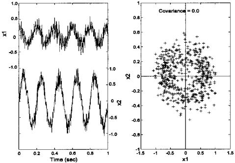
FIGURE 9.2 (A) Two waveforms made by mixing two sinusoids having different frequencies and amplitudes, then adding noise to the two mixtures. The resultant waveforms can be considered related variables since they both contain information from the same two sources. (B) The scatter plot of the two variables (or waveforms) was obtained by plotting one variable against the other for each point in time (i.e., each data sample). The correlation between the two samples (r = 0.77) can be seen in the diagonal clustering of points.

Since the data set was created using two separate sinusoidal sources, it should require two spatial dimensions. However, since each variable is composed of mixtures of the two sources, the variables have a considerable amount of covariance, or correlation.* Figure 9.2B is a scatter plot of the two variables, a plot of x1 against x2 for each point in time, and shows the correlation between the variables as a diagonal spread of the data points. (The correlation between the two variables is 0.77.) Thus, knowledge of the x value gives information on the

*Recall that covariance and correlation differ only in scaling. Definitions of these terms are given in Chapter 2 and are repeated for covariance below.

Copyright 2004 by Marcel Dekker, Inc. All Rights Reserved.

range of possible y values and vice versa. Note that the x value does not uniquely determine the y value as the correlation between the two variables is less than one. If the data were uncorrelated, the x value would provide no information on possible y values and vice versa. A scatter plot produced for such uncorrelated data would be roughly symmetrical with respect to both the horizontal and vertical axes.

For PCA to decorrelate the two variables, it simply needs to rotate the two-variable data set until the data points are distributed symmetrically about the mean. Figure 9.3B shows the results of such a rotation, while Figure 9.3A plots the time response of the transformed (i.e., rotated) variables. In the decorrelated condition, the variance is maximally distributed along the two orthogonal axes. In general, it may be also necessary to center the data by removing the means before rotation. The original variables plotted in Figure 9.2 had zero means so this step was not necessary.

While it is common in everyday language to take the word uncorrelated as meaning unrelated (and hence independent), this is not the case in statistical analysis, particularly if the variables are nonlinear. In the statistical sense, if two

FIGURE 9.3 (A) Principal components of the two variables shown in Figure 9.2. These were produced by an orthogonal rotation of the two variables. (B) The scatter plot of the rotated principal components. The symmetrical shape of the data indicates that the two new components are uncorrelated.

Copyright 2004 by Marcel Dekker, Inc. All Rights Reserved.

(or more) variables are independent they will also be uncorrelated, but the reverse is not generally true. For example, the two variables plotted as a scatter plot in Figure 9.4 are uncorrelated, but they are highly related and not independent. They are both generated by a single equation, the equation for a circle with noise added. Many other nonlinear relationships (such as the quadratic function) can generate related (i.e., not independent) variables that are uncorrelated. Conversely, if the variables have a Gaussian distribution (as in the case of most noise), then when they are uncorrelated they are also independent. Note that most signals do not have a Gaussian distribution and therefore are not likely to be independent after they have been decorrelated using PCA. This is one of the reasons why the principal components are not usually meaningful variables: they are still mixtures of the underlying sources. This inability to make two signals independent through decorrelation provides the motivation for the methodology known as independent component analysis described later in this chapter.

If only two variables are involved, the rotation performed between Figure 9.2 and Figure 9.3 could be done by trial and error: simply rotate the data until

FIGURE 9.4 Time and scatter plots of two variables that are uncorrelated, but not independent. In fact, the two variables were generated by a single equation for a circle with added noise.

Copyright 2004 by Marcel Dekker, Inc. All Rights Reserved.

the covariance (or correlation) goes to zero. An example of this approach is given as an exercise in the problems. A better way to achieve zero correlation is to use a technique from linear algebra that generates a rotation matrix that reduces the covariance to zero. A well-known technique exists to reduce a matrix that is positive-definite (as is the covariance matrix) into a diagonal matrix by preand post-multiplication with an orthonormal matrix (Jackson, 1991):

where S is the m-by-m covariance matrix, D is a diagonal matrix, and U is an orthonormal matrix that does the transformation. Recall that a diagonal matrix has zeros for the off-diagonal elements, and it is the off-diagonal elements that correspond to covariance in the covariance matrix (Eq. (19) in Chapter 2 and repeated as Eq. (5) below). The covariance matrix is defined by:

Hence, the rotation implied by U will produce a new covariance matrix, D, that has zero covariance. The diagonal elements of D are the variances of the new data, more generally known as the characteristic roots, or eigenvalues, of S: λ1, λ2, . . . λn. The columns of U are the characteristic vectors, or eigenvectors u1, u2, . . . un. Again, the eigenvalues of the new covariance matrix, D, correspond to the variances of the rotated variables (now called the principle components). Accordingly, these eigenvalues (variances) can be used to determine what percentage of the total variance (which is equal to the sum of all eigenvalues) a given principal component represents. As shown below, this is a measure of the associated principal component’s importance, at least with regard to how much of the total information it represents.

The eigenvalues or roots can be solved by the following determinant equa-

tion:

where I is the identity matrix. After solving for λ, the eigenvectors can be solved using the equation:

Copyright 2004 by Marcel Dekker, Inc. All Rights Reserved.

This approach can be carried out by hand for two or three variables, but is very tedious for more variables or long data sets. It is much easier to use singular value composition which has the advantage of working directly from the data matrix and can be done in one step. Moreover, singular value decomposition can be easily implemented with a single function call in MATLAB. Singular value decomposition solves an equation similar to Eq. (4), specifically:

In the case of PCA, X is the data matrix that is decomposed into (1) D, the diagonal matrix that contains, in this case, the square root of the eigenvalues; and (2) U, the principle components matrix. An example of this approach is given in the next section on MATLAB Implementation.

Order Selection

The eigenvalues describe how much of the variance is accounted for by the associated principal component, and when singular value decomposition is used, these eigenvalues are ordered by size; that is: λ1 > λ2 > λ3 . . . > λM. They can be very helpful in determining how many of the components are really significant and how much the data set can be reduced. Specifically, if several eigenvalues are zero or close to zero, then the associated principal components contribute little to the data and can be eliminated. Of course, if the eigenvalues are identically zero, then the associated principal component should clearly be eliminated, but where do you make the cut when the eigenvalues are small, but nonzero? There are two popular methods for determining eigenvalue thresholds. (1) Take the sum of all eigenvectors (which must account for all the variance), then delete those eigenvalues that fall below some percentage of that sum. For example, if you want the remaining variables to account for 90% of the variance, then chose a cutoff eigenvalue where the sum of all lower eigenvalues is less than 10% of the total eigenvalue sum. (2) Plot the eigenvalues against the order number, and look for breakpoints in the slope of this curve. Eigenvalues representing noise should not change much in value and, hence, will plot as a flatter slope when plotted against eigenvalue number (recall the eigenvalues are in order of large to small). Such a curve was introduced in Chapter 5 and is known as the scree plot (see Figure 5.6 D) These approaches are explored in the first example of the following section on MATLAB Implementation.

MATLAB Implementation

Data Rotation

Many multivariate techniques rotate the data set as part of their operation. Imaging also uses data rotation to change the orientation of an object or image.

Copyright 2004 by Marcel Dekker, Inc. All Rights Reserved.

From basic trigonometry, it is easy to show that, in two dimensions, rotation of a data point (x1, y1) can be achieved by multiplying the data points by the sines and cosines of the rotation angle:

where θ is the angle through which the data set is rotated in radians. Using matrix notation, this operation can be done by multiplying the data matrix by a rotation matrix:

This is the strategy used by the routine rotation given in Example 9.1 below. The generalization of this approach to three or more dimensions is straightforward. In PCA, the rotation is done by the algorithm as described below so explicit rotation is not required. (Nonetheless, it is required for one of the problems at the end of this chapter, and later in image processing.) An example of the application of rotation in two dimensions is given in the example.

Example 9.1 This example generate two cycles of a sine wave and rotate the wave by 45 deg.

Solution: The routine below uses the function rotation to perform the rotation. This function operates only on two-dimensional data. In addition to multiplying the data set by the matrix in Eq. (12), the function rotation checks the input matrix and ensures that it is in the right orientation for rotation with the variables as columns of the data matrix. (It assumes two-dimensional data, so the number of columns, i.e., number of variables, should be less than the number of rows.)

%Example 9.1 and Figure 9.5

%Example of data rotation

%Create a two variable data set of y = sin (x)

%then rotate the data set by an angle of 45 deg

clear all; close all;

Copyright 2004 by Marcel Dekker, Inc. All Rights Reserved.

FIGURE 9.5 A two-cycle sine wave is rotated 45 deg. using the function rotation that implements Eq. (12).

The rotation is performed by the function rotation following Eq. (12).

%Function rotation

%Rotates the first argument by an angle phi given in the second

%argument function out = rotate(input,phi)

%Input variables

Copyright 2004 by Marcel Dekker, Inc. All Rights Reserved.

% Set up rotation matrix

R = [cos(phi) sin(phi); -sin(phi) cos(phi)];

Principal Component Analysis Evaluation

PCA can be implemented using singular value decomposition. In addition, the MATLAB Statistics Toolbox has a special program, princomp, but this just implements the singular value decomposition algorithm. Singular value decomposition of a data array, X, uses:

[V,D,U] = svd(X);

where D is a diagonal matrix containing the eigenvalues and V contains the principal components in columns. The eigenvalues can be obtained from D using the diag command:

eigen = diag(D);

Referring to Eq. (9), these values will actually be the square root of the eigenvalues, λi. If the eigenvalues are used to measure the variance in the rotated principal components, they also need to be scaled by the number of points.

It is common to normalize the principal components by the eigenvalues so that different components can be compared. While a number of different normalizing schemes exist, in the examples here, we multiply the eigenvector by the square root of the associated eigenvalue since this gives rise to principal components that have the same value as a rotated data array (See Problem 1).

Example 9.2 Generate a data set with five variables, but from only two sources and noise. Compute the principal components and associated eigenvalues using singular value decomposition. Compute the eigenvalue ratios and generate the scree plot. Plot the significant principal components.

%Example 9.2 and Figures 9.6, 9.7, and 9.8

%Example of PCA

%Create five variable waveforms from only two signals and noise

%Use this in PCA Analysis

%

% Assign constants

Copyright 2004 by Marcel Dekker, Inc. All Rights Reserved.

FIGURE 9.6 Plot of eigenvalue against component number, the scree plot. Since the eigenvalue represents the variance of a given component, it can be used as a measure of the amount of information the associated component represents. A break is seen at 2, suggesting that only the first two principal components are necessary to describe most of the information in the data.

%

% Combine data in different proportions D(1,:) = .5*y .5*x .1*rand(1,N); D(2,:) = .2*y .7*x .1*rand(1,N); D(3,:) = .7*y .2*x .1*rand(1,N); D(4,:) = -.6*y -.24*x .2*rand(1,N);

Copyright 2004 by Marcel Dekker, Inc. All Rights Reserved.

FIGURE 9.7 Plot of the five variables used in Example 9.2. They were all produced from only two sources (see Figure 9.8B) and/or noise. (Note: one of the variables is pure noise.)

% way to do this

end

%

% Find Principal Components

[U,S,pc]= svd(D,0); % Singular value decompo-

% sition

Copyright 2004 by Marcel Dekker, Inc. All Rights Reserved.