Biosignal and Biomedical Image Processing MATLAB based Applications - John L. Semmlow

provide the most accurate determination of those features. Two spectral features of potential interest are the overall shape of the spectrum, termed the spectral estimate, and/or local features of the spectrum sometimes referred to as parametric estimates. For example, signal detection, finding a narrowband signal in broadband noise, would require a good estimate of local features. Unfortunately, techniques that provide good spectral estimation are poor local estimators and vice versa. Figure 3.2A shows the spectral estimate obtained by applying the traditional Fourier transform to a waveform consisting of a 100 Hz sine wave buried in white noise. The SNR is minus 14 db; that is, the signal amplitude is 1/5 of the noise. Note that the 100 Hz sin wave is readily identified as a peak in the spectrum at that frequency. Figure 3.2B shows the spectral estimate obtained by a smoothing process applied to the same signal (the Welch method, described later in this chapter). In this case, the waveform was divided into 32

FIGURE 3.2 Spectra obtained from a waveform consisting of a 100 Hz sine wave and white noise using two different methods. The Fourier transform method was used to produce the left-hand spectrum and the spike at 100 Hz is clearly seen. An averaging technique was used to create the spectrum on the right side, and the 100 Hz component is no longer visible. Note, however, that the averaging technique produces a better estimate of the white noise spectrum. (The spectrum of white noise should be flat.)

Copyright 2004 by Marcel Dekker, Inc. All Rights Reserved.

segments, the Fourier transform was applied to each segment, then the 32 spectra were averaged. The resulting spectrum provides a more accurate representation of the overall spectral features (predominantly those of the white noise), but the 100 Hz signal is lost. Figure 3.2 shows that the smoothing approach is a good spectral estimator in the sense that it provides a better estimate of the dominant noise component, but it is not a good signal detector.

The classical procedures for spectral estimation are described in this chapter with particular regard to their strengths and weaknesses. These methods can be easily implemented in MATLAB as described in the following section. Modern methods for spectral estimation are covered in Chapter 5.

THE FOURIER TRANSFORM: FOURIER SERIES ANALYSIS

Periodic Functions

Of the many techniques currently in vogue for spectral estimation, the classical Fourier transform (FT) method is the most straightforward. The Fourier transform approach takes advantage of the fact that sinusoids contain energy at only one frequency. If a waveform can be broken down into a series of sines or cosines of different frequencies, the amplitude of these sinusoids must be proportional to the frequency component contained in the waveform at those frequencies.

From Fourier series analysis, we know that any periodic waveform can be represented by a series of sinusoids that are at the same frequency as, or multiples of, the waveform frequency. This family of sinusoids can be expressed either as sines and cosines, each of appropriate amplitude, or as a single sine wave of appropriate amplitude and phase angle. Consider the case where sines and cosines are used to represent the frequency components: to find the appropriate amplitude of these components it is only necessary to correlate (i.e., multiply) the waveform with the sine and cosine family, and average (i.e., integrate) over the complete waveform (or one period if the waveform is periodic). Expressed as an equation, this procedure becomes:

where T is the period or time length of the waveform, fT = 1/T, and m is set of integers, possibly infinite: m = 1, 2, 3, . . . , defining the family member. This gives rise to a family of sines and cosines having harmonically related frequencies, mfT.

In terms of the general transform discussed in Chapter 2, the Fourier series analysis uses a probing function in which the family consists of harmonically

Copyright 2004 by Marcel Dekker, Inc. All Rights Reserved.

related sinusoids. The sines and cosines in this family have valid frequencies only at values of m/T, which is either the same frequency as the waveform (when m = 1) or higher multiples (when m > 1) that are termed harmonics. Since this approach represents waveforms by harmonically related sinusoids, the approach is sometimes referred to as harmonic decomposition. For periodic functions, the Fourier transform and Fourier series constitute a bilateral transform: the Fourier transform can be applied to a waveform to get the sinusoidal components and the Fourier series sine and cosine components can be summed to reconstruct the original waveform:

Note that for most real waveforms, the number of sine and cosine components that have significant amplitudes is limited, so that a finite, sometimes fairly short, summation can be quite accurate. Figure 3.3 shows the construction

FIGURE 3.3 Two periodic functions and their approximations constructed from a limited series of sinusoids. Upper graphs: A square wave is approximated by a series of 3 and 6 sine waves. Lower graphs: A triangle wave is approximated by a series of 3 and 6 cosine waves.

Copyright 2004 by Marcel Dekker, Inc. All Rights Reserved.

of a square wave (upper graphs) and a triangle wave (lower graphs) using Eq.

(3) and a series consisting of only 3 (left side) or 6 (right side) sine waves. The reconstructions are fairly accurate even when using only 3 sine waves, particularly for the triangular wave.

Spectral information is usually presented as a frequency plot, a plot of sine and cosine amplitude vs. component number, or the equivalent frequency. To convert from component number, m, to frequency, f, note that f = m/T, where T is the period of the fundamental. (In digitized signals, the sampling frequency can also be used to determine the spectral frequency). Rather than plot sine and cosine amplitudes, it is more intuitive to plot the amplitude and phase angle of a sinusoidal wave using the rectangular-to-polar transformation:

where C = (a2 + b2)1/2 and Θ = tan−1(b/a).

Figure 3.4 shows a periodic triangle wave (sometimes referred to as a sawtooth), and the resultant frequency plot of the magnitude of the first 10 components. Note that the magnitude of the sinusoidal component becomes quite small after the first 2 components. This explains why the triangle function can be so accurately represented by only 3 sine waves, as shown in Figure 3.3.

FIGURE 3.4 A triangle or sawtooth wave (left) and the first 10 terms of its Fourier series (right). Note that the terms become quite small after the second term.

Copyright 2004 by Marcel Dekker, Inc. All Rights Reserved.

Symmetry

Some waveforms are symmetrical or anti-symmetrical about t = 0, so that one or the other of the components, a(k) or b(k) in Eq. (3), will be zero. Specifically, if the waveform has mirror symmetry about t = 0, that is, x(t) = x(−t), than multiplications by a sine functions will be zero irrespective of the frequency, and this will cause all b(k) terms to be zeros. Such mirror symmetry functions are termed even functions. Similarly, if the function has anti-symmetry, x(t) = −x(t), a so-called odd function, then all multiplications with cosines of any frequency will be zero, causing all a(k) coefficients to be zero. Finally, functions that have half-wave symmetry will have no even coefficients, and both a(k) and b(k) will be zero for even m. These are functions where the second half of the period looks like the first half flipped left to right; i.e., x(t) = x(T − t). Functions having half-wave symmetry can also be either odd or even functions. These symmetries are useful for reducing the complexity of solving for the coefficients when such computations are done manually. Even when the Fourier transform is done on a computer (which is usually the case), these properties can be used to check the correctness of a program’s output. Table 3.1 summarizes these properties.

Discrete Time Fourier Analysis

The discrete-time Fourier series analysis is an extension of the continuous analysis procedure described above, but modified by two operations: sampling and windowing. The influence of sampling on the frequency spectra has been covered in Chapter 2. Briefly, the sampling process makes the spectra repetitive at frequencies mfT (m = 1,2,3, . . . ), and symmetrically reflected about these frequencies (see Figure 2.9). Hence the discrete Fourier series of any waveform is theoretically infinite, but since it is periodic and symmetric about fs /2, all of the information is contained in the frequency range of 0 to fs /2 ( fs /2 is the Nyquist frequency). This follows from the sampling theorem and the fact that the original analog waveform must be bandlimited so that its highest frequency, fMAX, is <fs /2 if the digitized data is to be an accurate representation of the analog waveform.

TABLE 3.1 Function Symmetries

Copyright 2004 by Marcel Dekker, Inc. All Rights Reserved.

The digitized waveform must necessarily be truncated at least to the length of the memory storage array, a process described as windowing. The windowing process can be thought of as multiplying the data by some window shape (see Figure 2.4). If the waveform is simply truncated and no further shaping is performed on the resultant digitized waveform (as is often the case), then the window shape is rectangular by default. Other shapes can be imposed on the data by multiplying the digitized waveform by the desired shape. The influence of such windowing processes is described in a separate section below.

The equations for computing Fourier series analysis of digitized data are the same as for continuous data except the integration is replaced by summation. Usually these equations are presented using complex variables notation so that both the sine and cosine terms can be represented by a single exponential term using Euler’s identity:

(Note mathematicians use i to represent √−1 while engineers use j; i is reserved for current.) Using complex notation, the equation for the discrete Fourier transform becomes:

n=0

where N is the total number of points and m indicates the family member, i.e., the harmonic number. This number must now be allowed to be both positive and negative when used in complex notation: m = −N /2, . . . , N /2–1. Note the similarity of Eq. (6) with Eq. (8) of Chapter 2, the general transform in discrete form. In Eq. (6), fm(n) is replaced by e−j2πmn/N. The inverse Fourier transform can be calculated as:

Applying the rectangular-to-polar transformation described in Eq. (4), it is also apparent *X(m)* gives the magnitude for the sinusoidal representation of the Fourier series while the angle of X(m) gives the phase angle for this representation, since X(m) can also be written as:

As mentioned above, for computational reasons, X(m) must be allowed to have both positive and negative values for m; negative values imply negative frequencies, but these are only a computational necessity and have no physical meaning. In some versions of the Fourier series equations shown above, Eq. (6)

Copyright 2004 by Marcel Dekker, Inc. All Rights Reserved.

is multiplied by Ts (the sampling time) while Eq. (7) is divided by Ts so that the sampling interval is incorporated explicitly into the Fourier series coefficients. Other methods of scaling these equations can be found in the literature.

The discrete Fourier transform produces a function of m. To convert this to frequency note that:

where f1 ≡ fT is the fundamental frequency, Ts is the sample interval; fs is the sample frequency; N is the number of points in the waveform; and TP = NTs is the period of the waveform. Substituting m = fmTs into Eq. (6), the equation for the discrete Fourier transform (Eq. (6)) can also be written as:

n=0

which may be more useful in manual calculations.

If the waveform of interest is truly periodic, then the approach described above produces an accurate spectrum of the waveform. In this case, such analysis should properly be termed Fourier series analysis, but is usually termed Fourier transform analysis. This latter term more appropriately applies to aperiodic or truncated waveforms. The algorithms used in all cases are the same, so the term Fourier transform is commonly applied to all spectral analyses based on decomposing a waveform into sinusoids.

Originally, the Fourier transform or Fourier series analysis was implemented by direct application of the above equations, usually using the complex formulation. Currently, the Fourier transform is implemented by a more computationally efficient algorithm, the fast Fourier transform (FFT), that cuts the number of computations from N 2 to 2 log N, where N is the length of the digital data.

Aperiodic Functions

If the function is not periodic, it can still be accurately decomposed into sinusoids if it is aperiodic; that is, it exists only for a well-defined period of time, and that time period is fully represented by the digitized waveform. The only difference is that, theoretically, the sinusoidal components can exist at all frequencies, not just multiple frequencies or harmonics. The analysis procedure is the same as for a periodic function, except that the frequencies obtained are really only samples along a continuous frequency spectrum. Figure 3.5 shows the frequency spectrum of a periodic triangle wave for three different periods. Note that as the period gets longer, approaching an aperiodic function, the spectral shape does not change, but the points get closer together. This is reasonable

Copyright 2004 by Marcel Dekker, Inc. All Rights Reserved.

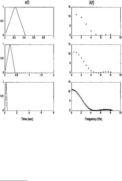
FIGURE 3.5 A periodic waveform having three different periods: 2, 2.5, and 8 sec. As the period gets longer, the shape of the frequency spectrum stays the same but the points get closer together.

since the space between the points is inversely related to the period (m/ T ).* In the limit, as the period becomes infinite and the function becomes truly aperiodic, the points become infinitely close and the curve becomes continuous. The analysis of waveforms that are not periodic and that cannot be completely represented by the digitized data is described below.

*The trick of adding zeros to a waveform to make it appear to a have a longer period (and, therefore, more points in the frequency spectrum) is another example of zero padding.

Copyright 2004 by Marcel Dekker, Inc. All Rights Reserved.

Frequency Resolution

From the discrete Fourier series equation above (Eq. (6)), the number of points produced by the operation is N, the number of points in the data set. However, since the spectrum produced is symmetrical about the midpoint, N/2 (or fs /2 in frequency), only half the points contain unique information.* If the sampling time is Ts, then each point in the spectra represents a frequency increment of 1/(NTs). As a rough approximation, the frequency resolution of the spectra will be the same as the frequency spacing, 1/(NTs). In the next section we show that frequency resolution is also influenced by the type of windowing that is applied to the data.

As shown in Figure 3.5, frequency spacing of the spectrum produced by the Fourier transform can be decreased by increasing the length of the data, N. Increasing the sample interval, Ts, should also improve the frequency resolution, but since that means a decrease in fs, the maximum frequency in the spectra, fs /2 is reduced limiting the spectral range. One simple way of increasing N even after the waveform has been sampled is to use zero padding, as was done in Figure 3.5. Zero padding is legitimate because the undigitized portion of the waveform is always assumed to be zero (whether true or not). Under this assumption, zero padding simply adds more of the unsampled waveform. The zero-padded waveform appears to have improved resolution because the frequency interval is smaller. In fact, zero padding does not enhance the underlying resolution of the transform since the number of points that actually provide information remains the same; however, zero padding does provide an interpolated transform with a smoother appearance. In addition, it may remove ambiguities encountered in practice when a narrowband signal has a center frequency that lies between the 1/NTs frequency evaluation points (compare the upper two spectra in Figure 3.5). Finally, zero padding, by providing interpolation, can make it easier to estimate the frequency of peaks in the spectra.

Truncated Fourier Analysis: Data Windowing

More often, a waveform is neither periodic or aperiodic, but a segment of a much longer—possibly infinite—time series. Biomedical engineering examples are found in EEG and ECG analysis where the waveforms being analyzed continue over the lifetime of the subject. Obviously, only a portion of such waveforms can be represented in the finite memory of the computer, and some attention must be paid to how the waveform is truncated. Often a segment is simply

*Recall that the Fourier transform contains magnitude and phase information. There are N/2 unique magnitude data points and N/2 unique phase data points, so the same number of actual data points is required to fully represent the data. Both magnitude and phase data are required to reconstruct the original time function, but we are often only interested in magnitude data for analysis.

Copyright 2004 by Marcel Dekker, Inc. All Rights Reserved.

cut out from the overall waveform; that is, a portion of the waveform is truncated and stored, without modification, in the computer. This is equivalent to the application of a rectangular window to the overall waveform, and the analysis is restricted to the windowed portion of the waveform. The window function for a rectangular window is simply 1.0 over the length of the window, and 0.0 elsewhere, (Figure 3.6, left side). Windowing has some similarities to the sampling process described previously and has well-defined consequences on the resultant frequency spectrum. Window shapes other than rectangular are possible simply by multiplying the waveform by the desired shape (sometimes these shapes are referred to as tapering functions). Again, points outside the window are assumed to be zero even if it is not true.

When a data set is windowed, which is essential if the data set is larger than the memory storage, then the frequency characteristics of the window become part of the spectral result. In this regard, all windows produce artifact. An idea of the artifact produced by a given window can be obtained by taking the Fourier transform of the window itself. Figure 3.6 shows a rectangular window on the left side and its spectrum on the right. Again, the absence of a window function is, by default, a rectangular window. The rectangular window, and in fact all windows, produces two types of artifact. The actual spectrum is widened by an artifact termed the mainlobe, and additional peaks are generated termed

FIGURE 3.6 The time function of a rectangular window (left) and its frequency characteristics (right).

Copyright 2004 by Marcel Dekker, Inc. All Rights Reserved.