Biosignal and Biomedical Image Processing MATLAB based Applications - John L. Semmlow

FIGURE 4.13 The magnitude and phase frequency response of a Parks–McClel- lan bandstop filter produced in Example 4.5. The number of filter coefficients as determined by remezord was 24.

% Now specify the deviation converting from db to linear dev = [(10v(rp_pass/20)-1)/(10v(rp_pass/20) 1) 10v

(-rp_stop/20)....(10v(rp_pass/20)-1)/(10v(rp_pass/ 20) 1)];

In Example 4.5 the vector assignment for the a vector is straightforward: the desired gain is given as 1 in the passband and 0 in the stopband. The actual stopband attenuation is given by the vector that specifies the maximum desirable

Copyright 2004 by Marcel Dekker, Inc. All Rights Reserved.

error, the dev vector. The specification of this vector, is complicated by the fact that it must be given in linear units while the ripple and stopband gain are specified in db. The db to linear conversion is included in the dev assignment. Note the complicated way in which the passband gain must be assigned.

Figure 4.13 shows the plot produced by freqz with no output arguments, a = 1, n = 512 (the default), and b was the FIR coefficient function produced in Example 4.6 above. The phase plot demonstrates the linear phase characteristics of this FIR filter in the passband. This will be compared with the phase characteristics of IIR filter in the next section.

The frequency response curves for Figure 4.13 were generated using the MATLAB routine freqz, which applies the FFT to the filter coefficients following Eq. (7). It is also possible to generate these curves by passing white noise through the filter and computing the spectral characteristics of the output. A comparison of this technique with the direct method used above is found in Problem 1.

Example 4.6 Design a differentiator using the MATLAB FIR filter remez. Use a two-stage design process (i.e., select a 28-order filter and bypass the first stage design routine remezord). Compare the derivative produced by this signal with that produced by the two-point central difference algorithm. Plot the results in Figure 4.14.

The FIR derivative operator will be designed by requesting a linearly increasing frequency characteristic (slope = 1) up to some fc Hz, then a sharp drop off within the next 0.1fs/2 Hz. Note that to make the initial magnitude slope equal to 1, the magnitude value at fc should be: fc * fs * π.

%Example 4.6 and Figure 4.14

%Design a FIR derivative filter and compare it to the

%Two point central difference algorithm

%

close all; clear all; load sig1;

Ts = 1/200; fs = 1/Ts; order = 28; L = 4;

fc = .05

t = (1:length(data))*Ts;

%

% Design filter

f = [ 0 fc fc .1 .9];

Copyright 2004 by Marcel Dekker, Inc. All Rights Reserved.

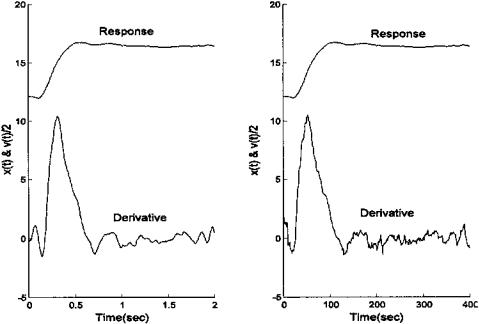
FIGURE 4.14 Derivative produced by an FIR filter (left) and the two-point central difference differentiator (right). Note that the FIR filter does produce a cleaner derivative without reducing the value of the peak velocity. The FIR filter order (n = 28) and deriviative cutoff frequency (fc = .05 fs/2) were chosen empirically to produce a clean derivative with a maximal velocity peak. As in Figure 4.5 the velocity (i.e., derivative) was scaled by 1/2 to be more compatible with response amplitude.

Copyright 2004 by Marcel Dekker, Inc. All Rights Reserved.

%

%

% Now apply two-point central difference algorithm

IIR Filters

IIR filter design under MATLAB follows the same procedures as FIR filter design; only the names of the routines are different. In the MATLAB Signal Processing Toolbox, the three-stage design process is supported for most of the IIR filter types; however, as with FIR design, the first stage can be bypassed if the desired filter order is known.

The third stage, the application of the filter to the data, can be implemented using the standard filter routine as was done with FIR filters. A Signal Processing Toolbox routine can also be used to implement IIR filters given the filter coefficients:

y = filtfilt(b,a,x)

The arguments for filtfilt are identical to those in filter. The only difference is that filtfilt improves the phase performance of IIR filters by running the algorithm in both forward and reverse directions. The result is a filtered sequence that has zero-phase distortion and a filter order that is doubled. The downsides of this approach are that initial transients may be larger and the approach is inappropriate for many FIR filters that depend on phase response for proper operations. A comparison between the filter and filtfilt algorithms is made in the example below.

As with our discussion of FIR filters, the two-stage filter processes will be introduced first, followed by three-stage filters. Again, all filters can be implemented using a two-stage process if the filter order is known. This chapter concludes with examples of IIR filter application.

Copyright 2004 by Marcel Dekker, Inc. All Rights Reserved.

Two-Stage IIR Filter Design

The Yule–Walker recursive filter is the only IIR filter that is not supported by an order-selection routine (i.e., a three-stage design process). The design routine yulewalk allows for the specification of a general desired frequency response curve, and the calling structure is given on the next page.

[b,a] = yulewalk(n,f,m)

where n is the filter order, and m and f specify the desired frequency characteristic in a fairly straightforward way. Specifically, m is a vector of the desired filter gains at the frequencies specified in f. The frequencies in f are relative to fs/2: the first point in f must be zero and the last point 1. Duplicate frequency points are allowed and correspond to steps in the frequency response. Note that this is the same strategy for specifying the desired frequency response that was used by the FIR routines fir2 and firls (see Help file).

Example 4.7 Design an 12th-order Yule–Walker bandpass filter with cutoff frequencies of 0.25 and 0.5. Plot the frequency response of this filter and compare with that produced by the FIR filter fir2 of the same order.

%Example 4.7 and Figure 4.15

%Design a 12th-order Yulewalk filter and compare

%its frequency response with a window filter of the same

%order

xlabel(’Relative Frequency’);

Copyright 2004 by Marcel Dekker, Inc. All Rights Reserved.

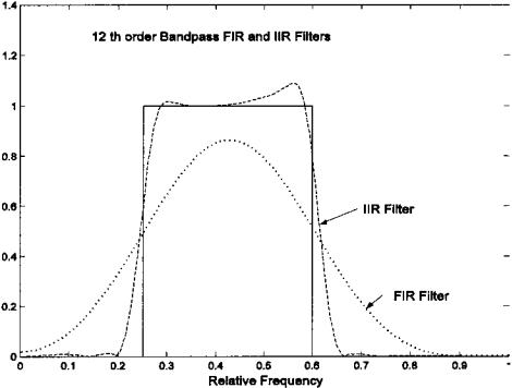
FIGURE 4.15 Comparison of the frequency response of 12th-order FIR and IIR filters. Solid line shows frequency characteristics of an ideal bandpass filter.

Three-Stage IIR Filter Design: Analog Style Filters

All of the analog filter types—Butterworth, Chebyshev, and elliptic—are supported by order selection routines (i.e., first-stage routines). The first-stage routines follow the nomenclature as FIR first-stage routines, they all end in ord. Moreover, they all follow the same strategy for specifying the desired frequency response, as illustrated using the Butterworth first-stage routine buttord:

[n,wn] = buttord(wp, ws, rp, rs); Butterworth filter

where wp is the passband frequency relative to fs/2, ws is the stopband frequency in the same units, rp is the passband ripple in db, and rs is the stopband ripple also in db. Since the Butterworth filter does not have ripple in either the passband or stopband, rp is the maximum attenuation in the passband and rs is the minimum attenuation in the stopband. This routine returns the output argu-

Copyright 2004 by Marcel Dekker, Inc. All Rights Reserved.

ments n, the required filter order and wn, the actual −3 db cutoff frequency. For example, if the maximum allowable attenuation in the passband is set to 3 db, then ws should be a little larger than wp since the gain must be less that 3 db at wp.

As with the other analog-based filters described below, lowpass, highpass, bandpass, and bandstop filters can be specified. For a highpass filter wp is greater than ws. For bandpass and bandstop filters, wp and ws are two-element vectors that specify the corner frequencies at both edges of the filter, the lower frequency edge first. For bandpass and bandstop filters, buttord returns wn as a two-element vector for input to the second-stage design routine, butter.

The other first-stage IIR design routines are:

The second-stage routines follow a similar calling structure, although the Butterworth does not have arguments for ripple. The calling structure for the Butterworth filter is:

[b,a] = butter(n,wn,’ftype’)

where n and wn are the order and cutoff frequencies respectively. The argument ftype should be ‘high’ if a highpass filter is desired and ‘stop’ for a bandstop filter. In the latter case wn should be a two-element vector, wn = [w1 w2], where w1 is the low cutoff frequency and w2 the high cutoff frequency. To specify a bandpass filter, use a two-element vector without the ftype argument. The output of butter is the b and a coefficients that are used in the third or application stage by routines filter or filtfilt, or by freqz for plotting the frequency response.

The other second-stage design routines contain additional input arguments to specify the maximum passband or stopband ripple if appropriate:

[b,a] = cheb1(n,rp,wn,’ftype’) % Chebyshev Type I filter

where the arguments are the same as in butter except for the additional argument, rp, which specifies the maximum desired passband ripple in db.

The Type II Chebyshev filter is:

Copyright 2004 by Marcel Dekker, Inc. All Rights Reserved.

where again the arguments are the same, except rs specifies the stopband ripple. As we have seen in FIR filters, the stopband ripple is given with respect to passband gain. For example a value of 40 db means that the ripple will not exceed 40 db below the passband gain. In effect, this value specifies the minimum attenuation in the stopband.

The elliptic filter includes both stopband and passband ripple values:

[b,a] = ellip(n,rp,rs,wn,’ftype’) % Elliptic filter

where the arguments presented are in the same manner as described above, with rp specifying the passband gain in db and rs specifying the stopband ripple relative to the passband gain.

The example below uses the second-stage routines directly to compare the frequency response of the four IIR filters discussed above.

Example 4.8 Plot the frequency response curves (in db) obtained from an 8th-order lowpass filter using the Butterworth, Chebyshev Type I and II, and elliptic filters. Use a cutoff frequency of 200 Hz and assume a sampling frequency of 2 kHz. For all filters, the passband ripple should be less than 3 db and the minimum stopband attenuation should be 60 db.

%Example 4.8 and Figure 4.16

%Frequency response of four 8th-order lowpass filters

Copyright 2004 by Marcel Dekker, Inc. All Rights Reserved.

FIGURE 4.16 Four different 8th-order IIR lowpass filters with a cutoff frequency of 200 Hz. Sampling frequency was 2 kHz.

Copyright 2004 by Marcel Dekker, Inc. All Rights Reserved.

PROBLEMS

1. Find the frequency response of a FIR filter with a weighting function of bn = [.2 .2 .2 .2 .2] in three ways: apply the FFT to the weighting function, use freqz, and pass white noise through the filter and plot the magnitude spectra of the output. In the third method, use a 1024-point array; i.e., y = filter (bn,1,randn(1024,1)). Note that you will have to scale the frequency axis differently to match the relative frequencies assumed by each method.

2.Use sig_noise to construct a 512-point array consisting of two closely spaced sinusoids of 200 and 230 Hz with SNR of −8 db and −12 db respectively. Plot the magnitude spectrum using the FFT. Now apply an 24 coefficient FIR bandpass window type filter to the data using either the approach in Example 4.2 or the fir1 MATLAB routine. Replot the bandpass filter data.

3.Use sig_noise to construct a 512-point array consisting of a single sinusoid of 200 Hz at an SNR of −20 db. Narrowband filter the data with an FIR rectangular window type filter, and plot the FFT spectra before and after filtering. Repeat using the Welch method to obtain the power spectrum before and after filtering.

4.Construct a 512-point array consisting of a step function. Filter the step by four different FIR lowpass filters and plot the first 150 points of the resultant

Copyright 2004 by Marcel Dekker, Inc. All Rights Reserved.